Disclaimer: This is Untrue.
2.6.11 Beyond the Standard Model
2.6.11.1 Overview
The Standard Model was established, but faced some difficulties.
Then the theory was improved one by one.
Firstly, Supersymmetric Theory was introduced.
The second step split into roughly 2 schools
in reference to continuous homogeneity of Spacetime or minimum units of Spacetime.
The 1st school based on the presumption that Spacetime is homogeneous continuum
and absence of minimun units.
In contrast, the 2nd school based on the
presumption that Spacetime is inhomogeneous and consists of components with
minimum units.
The 1st "absence of minimum units of Spacetime" school
had difficulties in integrating Gravity with infinities arising
in quantity calculation regardless of renormalization,
and managed to
propose Superstring Theory employing 10 or 11 dimensional Spacetime
supported by Supersymmetric Theory.
However, it seems mathematical fictional fantasy irrelevant to the General Theory of Relativity
as a whole.
Yet, the virtue of Superstring Theory might be seen in its multiverse theory.
The 2nd "presence of minimum units of Spacetime" school bore
"Loop Quantum Gravity" (and "Causal Dynamical Triangulation")
associated with the General Theory of Relativity.
Thus humans approached the final answer, the Whole Inclusive Theory of Everything.
2.6.11.2 Detals
2.6.11.2.1 Georgi and Dimopoulos's Minimal Supersymmetric Standard Model in 1981 CE
Background
The Standard Model was established, but it yet had some problems.
The 2 major problems claimed were 2 kinds of Hierarchy Problems,
"Hierarchy Problem about Forces" and
"Hierarchy Problem about the mass of Higgs particle."
"Hierarchy Problem about Forces" is the great difference between Gravity and other forces in strength.
Gravity is extraordinary weaker even than the weakest force of the other 3 forces,
10-32 times weaker than the Weak Force.
(The Electromagnetic Force is some 10-100 times weaker than the Strong Force.
(The precise ratio depends on the distances of the forces.)
The Weak Force is some 10 times weaker than Electromagnetic Force.)
"Hierarchy Problem
about the mass of Higgs particle" is that the experimentally estimated mass of Higgs particle
is rather smaller than theoretically estimated mass.
Collecting and summarizing primary constants in physics such as Planck Constant
and the speed of light,
it results in Planck Mass, 1.22*1019 GeV.
It implies the original mass or fundamental mass could be some 1019 GeV.
In contrast to that, bosons generally have light mass or no mass including Higgs Bosons.
For example, photons have no mass.
The mass of Higgs Boson was also experimentally estimated rather light,
around 100-200 GeV, at that time
from a viewpoint of mass of derived particles, employing particle accelerators,
supposedly from likely Higgs Bosons.
On the other hand, as mentioned before, the light mass or no mass of bosons
could be accounted for by
symmetry.
However, since the spin of Higgs Boson is 0, Higgs Bosons
wouldn't have symmetry according to the
Standard Model.
Higgs Bosons had no reason accounting for the light mass.
This Hierarchy Problem about Higgs Mass had to be resolved
introducing a new
theory.
*
"Hierarchy Problem in Wikipedia"
http://en.wikipedia.org/wiki/Hierarchy_problem
Minimal Supersymmetric Standard Model
Georgi and Dimopoulos presented Minimal Supersymmetric Standard Model
introducing Supersymmetric Theory simply to the Standard
Model assuming supersymmetric particles.
(Supersymmetric particles are frequently called "sparticles,"
preceded by "s" representing "supersymmetry.")
The assumption of Supersymmetry with supersymmetric particles
solves the Hierarchy Problem about Higgs Mass
Since the Supersymmetry assumes supersymmetric particles of Higgs Boson,
Symmetry of Higgs Bosons accounting for
the light mass of Higgs Bosons is assumed.
*
"Minimal Supersymmetric Standard Model in Wikipedia"
http://en.wikipedia.org/wiki/Minimal_Supersymmetric_Standard_Model
*
"Minimal Supersymmetric Standard Model Download"
http://arxiv.org/abs/hep-ph/9709356
In addition, the Supersymmetric Theory implied seemingly favorable presumption
in relation to the unification theory of the 3 forces.
The reciprocals of the coupling constant of the 3 forces and temperature/energy level
are illustrated as follows.
*
"Coupling Constant in Wikipedia"
http://en.wikipedia.org/wiki/Coupling_constant
According to the reciprocals based on the Standard Model, the reciprocals wouldn't
match at any energy level.
However, according to the reciprocals based on the Supersymmetric Theory,
the 3 reciprocals of the coupling constant might match at a specific high energy level.
It implies the 3 forces were originally unified based on the Supersymmetric Theory
implying the legitimacy of the Supersymmetric Theory.
Aside from that, according to the Supersymmetric Theory, Dark Matter could be identified with
some supersymmetric particles.
*As mentioned above, according to common physicists,
"Hierarchy Problem about Forces" is claimed as well.
However, it should be noted that the 3 forces (Strong Force, Electromagnetic Force,
and Weak Force)
and Gravity are different things based on different mechanisms.
The 3 forces are mediated by particles (Gluons, Virtual Quarks, Photons, and Weak Bosons).
However, as the General Theory of Relativity tells, Gravity is derived from curvatures of spacetime.
(Gravitons might curve spacetime.)
Gravitons wouldn't directly mediate Gravity.
Since the mechanisms are totally different, there would be
no problem involving "Hierarchy Problem about Forces."
2.6.11.2.2 Aspect's Quantum Entanglement Experiment in 1982 CE
2.6.11.2.2.1 Background
Quantum entanglement was originally proposed by Albert Einstein and his colleagues as a thought experiment to criticize the completeness of quantum mechanics. Their argument, known as Local Realism, asserted that physical phenomena occurring in a small region of space cannot influence phenomena in a distant region faster than the speed of light (Locality), and that physical properties exist independently of whether they are measured (Realism).
As mentioned before, in 1964 CE, John Bell formulated Bell's Inequality, providing a mathematical criterion to test local realism. Subsequent experiments, such as those by John Clauser in 1972 CE using calcium atoms, began to suggest that correlations between distant photons might indeed exist.
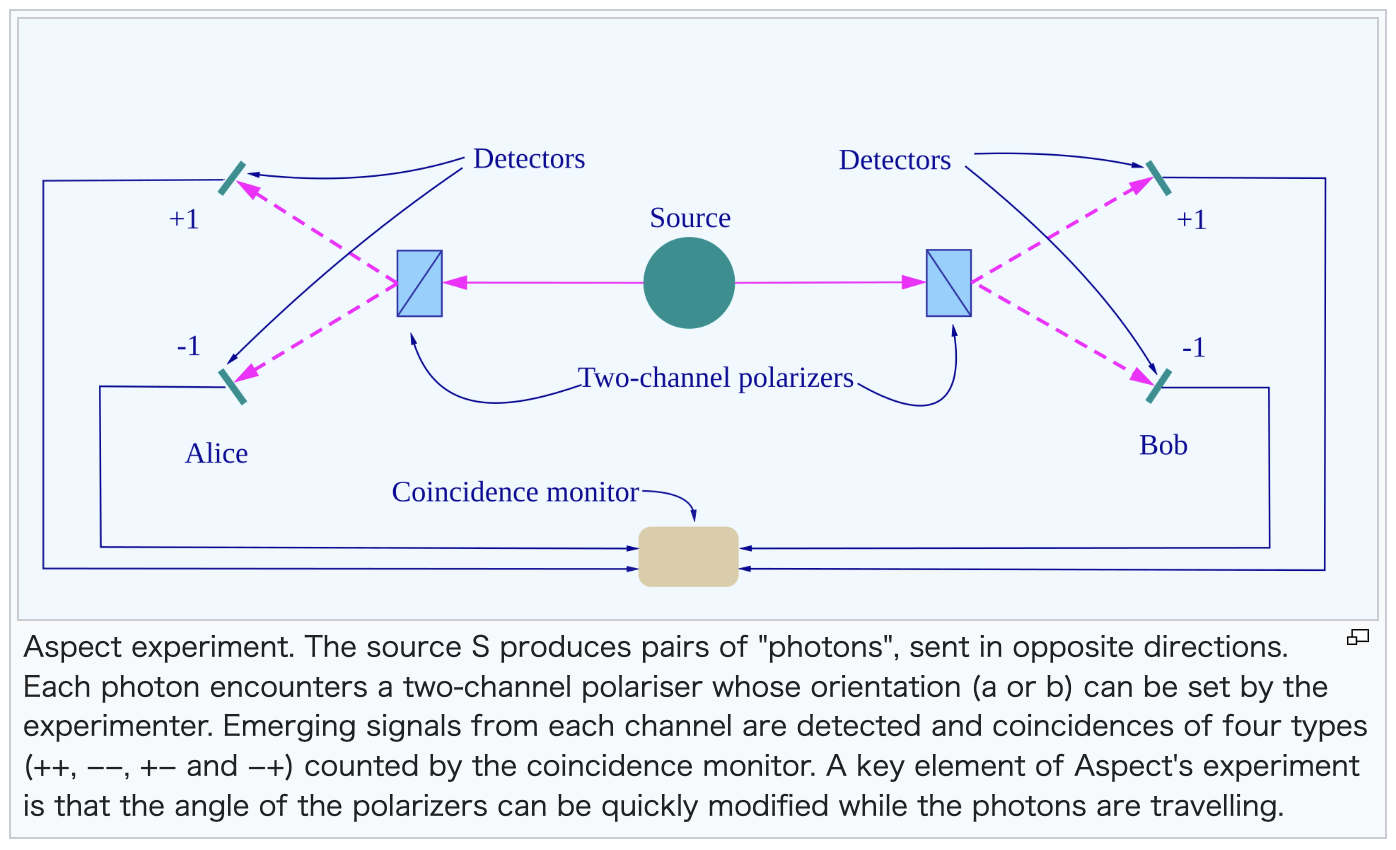
2.6.11.2.2.2 Aspect's Quantum Entanglement Experiment
2.6.11.2.2.2.1 Experimental Setup and Mechanism
Alain Aspect’s 1982 CE experiment significantly advanced Clauser’s work, providing the
definitive evidence.
The structure of Aspect's experiment is illustrated in the diagram below.
Traditionally, these phenomena are explained using the terminology of
particles such as electrons and photons. For the sake of convenience, these terms are used
here. However, please note that these are essentially labels or conceptual models applied to
fluctuations in the fabric of spacetime (waves in spacetime), and as such,
some technical nuances may be difficult to explain in exhaustive detail.
(1) The Source (S)
Calcium atoms are irradiated with lasers. In a calcium atom, the activity regions and energy states (electron orbitals) of the two outermost electrons are highly susceptible to change. Therefore, these two electrons transition their orbitals and enter an excited state.
Generally, when an electron undergoes accelerated motion or displacement, magnetic field lines are generated in a ring shape perpendicular to the direction of that movement. This phenomenon can also be described as the emission of a photon in the perpendicular direction.
When the laser irradiation to the calcium atom stops, the electrons return to their original ground state. As the first electron transitions, energy is released. Suppose this electron moves vertically from top to bottom; this generates an electric field that fluctuates in the same vertical direction.
Thus, the emission of a single photon results in an electric field that fluctuates in a direction vertical to the ground—that is, up and down.
What is commonly referred to as the "oscillation of a photon" actually refers, more precisely, to the oscillation of the electric field associated with the photon. The term "angle of a photon's oscillation" correctly refers to the angle of the electric field fluctuation caused by the photon.
In the experimental setup, if a photon is emitted toward A (Alice), it passes through a transparent medium consisting of water or tellurium dioxide crystals, as described later, and proceeds toward the detector.
(2) The Second Photon
Approximately 5 nanoseconds later, the second electron also returns from the excited state to the ground state, emitting a second photon. According to the law of conservation of angular momentum, the direction of the electric field fluctuation for the first and second photons must, in principle, be the same. Following the previous example, the second photon also results in an electric field fluctuating in the vertical direction (up and down).
To maintain the overall balance around the calcium atom, the second photon tends to be emitted in the opposite direction to the first one.
In the experimental setup, if a photon is emitted toward B (Bob), it passes through the other transparent medium consisting of water or tellurium dioxide crystals (which will be described in detail later) and proceeds toward the detector.
(3) The Polarizers
Immediately in front of the photon detectors at stations A (Alice) and B (Bob), polarizers are set to specific angles.
For example, a polarizer set at 0° relative to a vertical line to the ground allows vertically oscillating photons (those whose electric field fluctuation is vertical to the ground) to pass 100% while blocking horizontal ones.
A polarizer consists of an array of long molecules that conduct electrons. Setting a polarizer to 0° relative to the vertical line corresponds to aligning these long molecules horizontally. In this configuration, if the photon's electric field fluctuates horizontally, the electrons within the molecules oscillate, thereby absorbing the photon's energy and preventing it from passing. Conversely, if the photon's electric field fluctuates vertically, it does not interact with the molecules, allowing the photon to pass through.
For intermediate angles, the probability of passage follows Malus's Law ($P = \cos^2 \theta$). For instance, if the direction of the electric field oscillation is at 45° relative to the vertical line, the probability of the photon passing is $\cos^2 45^\circ = 1/2$.
At each station, A and B, a second detector is also installed, with a corresponding polarizer
set immediately in front of each.
(4) The Switching Mechanism
To enable advanced experimentation, Aspect’s setup equipped the acousto-optic cells (the water or tellurium dioxide crystals through which the photons pass) with acousto-optical switches. These switches were connected to piezoelectric transducers made of materials such as quartz or barium titanate.
The oscillations generated by the piezoelectric transducers rapidly fluctuate the density distribution within the cells. As a result, the photon's path changes randomly every 10 nanoseconds, making it unpredictable which polarizer the photon will enter.
(5) Scale of the Experimental Apparatus
Aspect set the distance between the source and the polarizers to approximately 6 meters (resulting in a total separation of 12 meters between Alice and Bob).
The time required for light to travel a distance of 6 meters is approximately 20 nanoseconds ($20 \times 10^{-9}$ seconds).
*Attribution:
"Aspect's Experiment on Wikipedia"
https://en.wikipedia.org/wiki/Aspect%27s_experiment
2.6.11.2.2.2.2 Experimental Verification and Findings
2.6.11.2.2.2.2.1 Experiment 1: The Static Setup — Testing the Baseline of Correlation
In the initial stage of the experiment, the piezoelectric transducers are kept inactive, allowing the photons to travel in a straight path through the transparent cells. Both polarizers at stations A and B are set to 0°. When the laser is repeatedly fired at the calcium atoms over many trials, the detector at station A will respond to a photon detection dozens or hundreds of times. In these instances, the detector at station B also responds with a probability nearly reaching 100%.
This phenomenon is difficult to explain from the perspective of Einsteinian Local Realism.
Since the two photons are supposed to be emitted with their electric fields oscillating in the same direction, consider a case where the photons' electric fields are oscillating at a 45° angle. The first photon (heading toward A) has a 50% probability of passing through its polarizer. However, the second photon (heading toward B) would also only have a 50% probability of passing. Local realism cannot explain why the detection of the first photon at A is accompanied by a nearly 100% detection rate of the second photon at B.
(Furthermore, if the oscillation directions of the two photons were determined independently, it would be even more impossible to explain this perfect correlation.)
A similar phenomenon was observed in John Clauser's 1972 experiment. (However, Clauser's setup was smaller in scale and did not utilize transparent crystals like tellurium dioxide.) Clauser's findings cast doubt on local realism. Proponents of local realism might first argue that when the first photon passes the polarizer or hits the detector, that information travels at or below the speed of light to the second photon, which then adjusts its oscillation direction accordingly. In a small-scale setup, if the distance from the calcium source to the polarizers is short, such information could potentially return within 5 nanoseconds—before the second photon is fully emitted.
However, in Aspect’s experiment, a 6-meter distance was maintained between the calcium source and the polarizers, a distance that requires 20 nanoseconds to travel even at the speed of light.
Since the second photon is emitted approximately 5 nanoseconds after the first, it is impossible for information to
be transmitted to the second photon at the speed of light.
2.6.11.2.2.2.2.2 Potential Counter-argument from Local Realism: "Residual Conditions in the Path"
To save local realism under these conditions, one might resort to the logic that "because the experiments were repeated with fixed polarizer angles, the measurement conditions lingered in the photons' path, allowing new photons to 'learn' these conditions and adjust their oscillation angles."
2.6.11.2.2.2.2.3 Experiment 2: The Dynamic Setup — High-Speed Randomized Switching
To eliminate this possibility, Aspect devised a method to change the polarizer angles randomly and at high speed. As the photons pass through the transparent cells, high-frequency oscillations fluctuate the density distribution of the crystals, randomly diverting the photons' paths into one of two directions. At the end of each path, polarizers and detectors set to different angles are waiting, ensuring the measurement settings are chosen only after the photons are already in flight.
The experimental results corresponding to the claims assumed by Local Realism are as follows.
The results can be classified into the following four patterns based on the combinations of angles at stations A and B. The values below represent the following parameters:
Alice’s Angle (A)
Bob’s Angle (B)
Angular Difference (θ)
Detection Probability at Bob (Pb )
(1)
$A_1 = 0^\circ$
$B_1 = 22.5^\circ$
Angular Difference (θ) $22.5^\circ$
Approx. 85%
(2)
$A_2 = 45^\circ$
$B_1 = 22.5^\circ$
Angular Difference (θ) $22.5^\circ$
Approx. 85%
(3)
$A_1 = 0^\circ$
$B_2 = 67.5^\circ$
Angular Difference (θ) $67.5^\circ$
Approx. 15%
(4)
$A_2 = 45^\circ$
$B_2 = 67.5^\circ$
Angular Difference (θ) $22.5^\circ$
Approx. 85%
2.6.11.2.2.2.2.4 Theoretical Interpretations
(i) The Quantum Mechanical View
When the first photon passes through Alice's polarizer, its state "collapses" to match that polarizer's angle. Instantly, the entangled second photon is "rewritten" into that same state.
Consequently, when it reaches Bob's polarizer:
In cases (1), (2), and (4): The photon faces a pure angular difference of $22.5^\circ$, yielding $\cos^2(22.5^\circ) \approx 85\%$.
In case (3): The photon faces a pure angular difference of $67.5^\circ$, yielding $\cos^2(67.5^\circ) \approx 15\%$.
This matches the experimental data perfectly.
(ii) The Local Realism (Classical) View
If we assume the photons have a pre-determined distribution ($P(\theta) \propto \cos^2 \theta$) and follow Malus's Law independently, the calculated probability for a 22.5° difference is only 67.7%. For a 67.5° difference, it is 32.3%. Both differ significantly from the results.
(iii) The "Best-Case" Classical Hypothesis
To bridge this gap, proponents of local realism might propose a Deterministic Hidden Variable Model: "Perhaps Malus's Law is a statistical illusion, and photons actually pass 100% if the angle is within $\pm45^\circ$ and 0% otherwise." Even with this extreme "all-or-nothing" advantage, the classical correlation only reaches 75% (for 22.5°) and 25% (for 67.5°), failing to reach the observed 85% and 15%.
2.6.11.2.2.3 Conclusion
The experimental value of the Bell parameter was measured at $S \approx 2.7$, which far exceeds the classical limit of $S \le 2$ and approaches the quantum maximum of 2.82. This confirms that local realism is untenable. Furthermore, it has been confirmed that there are phenomena that cannot be explained by conventional physical theories, including local realism and the special theory of relativity.
2.6.11.2.2.4 Further Findings
Subsequent experiments have estimated that if any "information" were being transmitted
between the photons, it would have to travel at over 10,000 times the speed of light.
In addition, there are reports that this quantum entanglement phenomenon has been
confirmed over distances as great as 1,200 km. This might suggest that the connection is
not a form of communication, but rather a manifestation of the fundamental non-locality
of the universe.
*
"Bell Test Experiments on Wikipedia"
http://en.wikipedia.org/wiki/Bell_test_experiments
*
"Nonlocality on Wikipedia"
http://en.wikipedia.org/wiki/Nonlocality
*
"Quantum Entanglement on Wikipedia"
https://en.wikipedia.org/wiki/Quantum_entanglement
2.6.11.2.3 Exotic Differentiable Structure of 4-Dimensional Space in 1983 CE
2.6.11.2.3.1 Outline
While our universe appears to consist of 3-dimensional space and 1-dimensional time, the underlying "context" or mathematical fabric remains elusive.
In 1982 CE, mathematician Simon Donaldson provided a profound clue through Donaldson’s Theorem.
When integrated with Freedman’s Theorem, it revealed a unique property of 4-dimensional Euclidean space ($R^4$) that exists nowhere else. Unlike Euclidean spaces of any other dimension, 4-dimensional space alone allows for what is called an "Exotic Differentiable Structure." In simpler terms, it is a structure that is topologically the same but "oddly subdivided" or smoothed in a way that defies standard geometric intuition.
*
"Exotic R4 in Wikipedia"
https://en.wikipedia.org/wiki/Exotic_R4
*
"4-Manifold in Wikipedia"
https://en.wikipedia.org/wiki/4-manifold
*
"Donaldson's Theorem in Wikipedia"
https://en.wikipedia.org/wiki/Donaldson%27s_theorem
To grasp the "Exotic Differentiable Structure" of 4D space, one must understand three key concepts: "manifolds," "homeomorphism," and "diffeomorphism." However, it should be noted that topology—including these three concepts—is fundamentally a mathematical framework (an idea) used to describe reality, rather than a physical entity itself.
2.6.11.2.3.2 Manifold
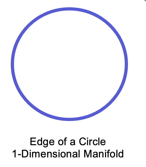
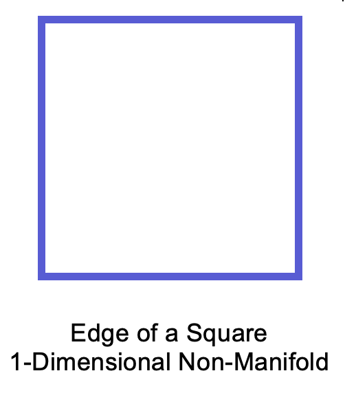
A manifold is a smooth object.
For example, the edge of a circle is 1-Dimensional manifold. The edge of a square is not 1-Dimensional manifold, since it has corners then it is not smooth.
The edge of a sphere (the surface of a sphere) is 2-Dimensional manifold. The edge of a cube (the surface of a cube) is not 2-Dimensional manifold.
Specifically, a manifold is defined as a topological space (an object) that satisfies two key properties:
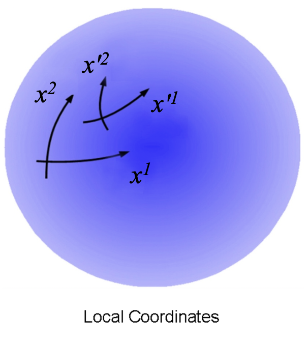
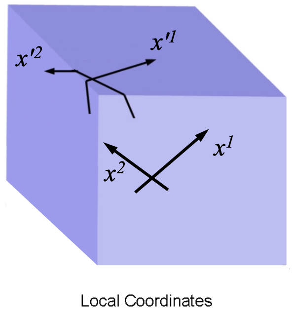
First, after determining the dimensionality of the topological space, for any point on the object, a local coordinate system (a chart) with that point as its origin should be established. This local coordinate system should match the dimensionality of the topological space (the object). For instance, if a 2-dimensional manifold is assumed in 3-dimensional Euclidean space, it is necessary to be able to set up a 2-dimensional coordinate system in the topological space centered at a given point. Furthermore, another local coordinate system of the same dimension which is centered at a point near the original point should be established in the topological space (the object) being defined through a transition function that is infinitely differentiable. ($C^\infty$ denotes infinite differentiability.)
Second, the inverse of this transition function should also be infinitely differentiable. In other words, the mapping from the second local coordinate system back to the original one (the inverse function) should be $C^\infty$ as well.
This bi-directional, infinitely differentiable mapping between coordinate systems is called a diffeomorphism.
Formally, these conditions imply that one can transition from a given coordinate system and its origin to a neighboring coordinate system and its origin through a smooth transformation. In essence, this means that the neighborhood of any given point is perfectly smooth. If this property holds for every point on the object, it signifies that the entire object is smooth. The object (the topological space) is called a manifold.
While a cube has local coordinates at every point, it fails to be a manifold because the transition functions at its edges and corners are not differentiable. In contrast, a manifold behaves locally like an infinitely flat plane, allowing for consistent calculus across its entire surface.
Note that a Euclidean space of the same dimension (an infinitely flat space where all axes are orthogonal to each other) satisfies these conditions and is therefore considered a manifold.
2.6.11.2.3.3 Homeomorphism in Coordinate Transformation
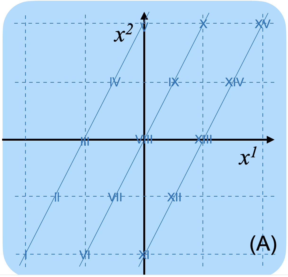
To illustrate how a coordinate system affects our perception of a shape, consider an original coordinate system $ x^1, x^2 $ and a new coordinate system $ x'^1, x'^2 $. (Here, $ x^1 $ and $ x'^1 $ represent the horizontal axis, while $ x^2 $ and $ x'^2 $ represent the vertical axis.)
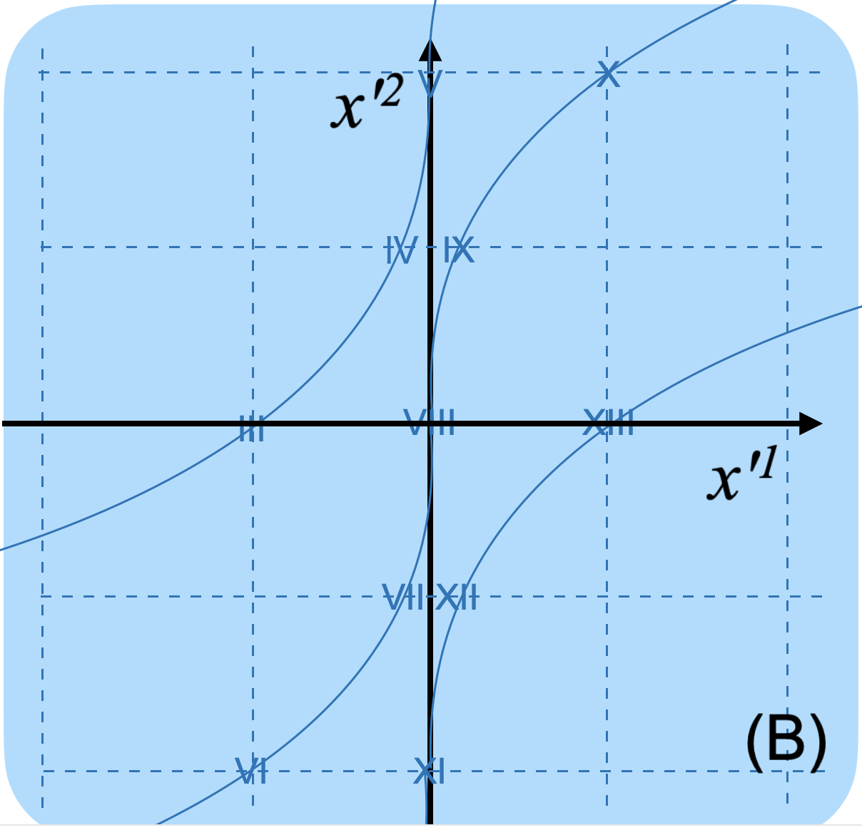
In this diagram, a transformation is assumed so that the horizontal axis is converted by the function $ x'^1 = (x^1)^3 $, while the vertical axis remains unchanged as $ x'^2 = x^2 $.
In this scenario, a simple diagonal line in the original $ x^1, x^2 $ coordinate system will appear as an S-shaped curve when plotted on the grid of the new $ x'^1, x'^2 $ coordinate system. In this transformation, lines that were originally continuous remain continuous after the transformation. This property, where continuity is preserved, is called a homeomorphism.
2.6.11.2.3.4 Diffeomorphism in Coordinate Transformation
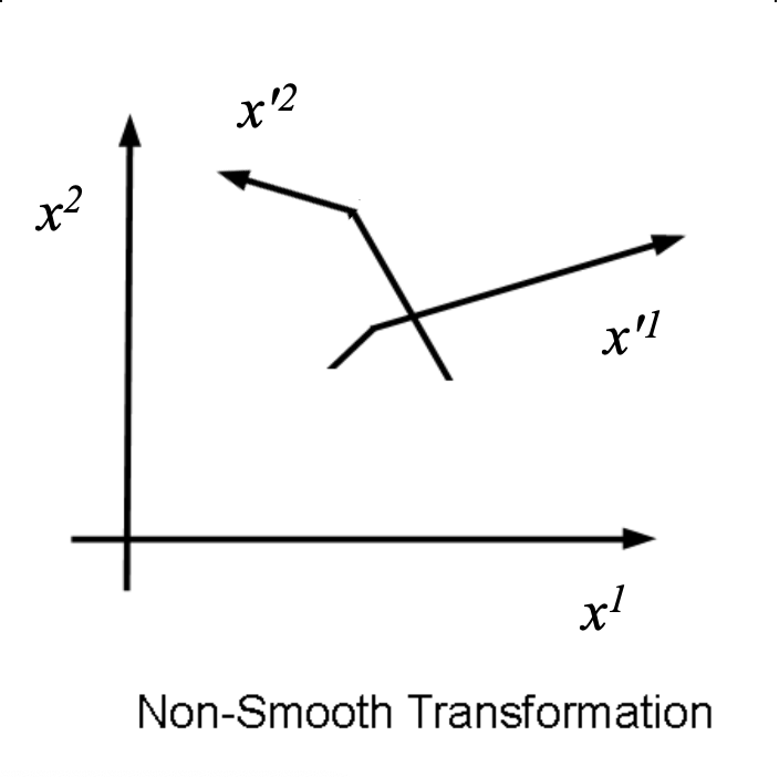
Furthermore, using elementary mathematics, the function $ x'^1 = (x^1)^3 $ can be differentiated with respect to $ x^1 $ three times; from the fourth derivative onwards, the result is always $ 0 $, meaning it can be differentiated infinitely many times. Thus, this transition function is $ C^\infty $.
However, its inverse function is $ x^1 = (x'^1)^{1/3} $, which cannot be differentiated with respect to $ x'^1 $ at $ x'^1 = 0 $. This is because the inverse function becomes vertical along the $ x'^1 $ axis at that point. Therefore, this specific transformation does not qualify as a diffeomorphism.
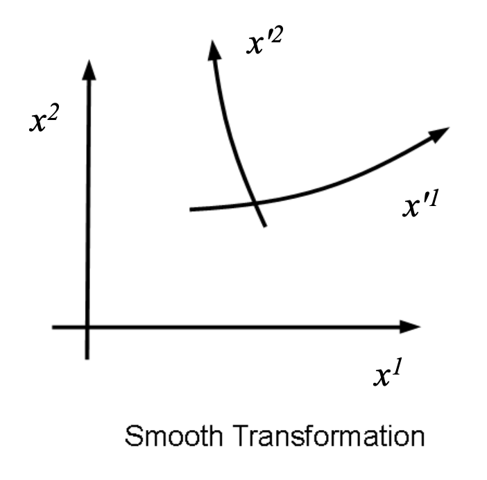
In the next example, a transformation is assumed so that the horizontal axis is converted by the function $ x'^1 = (x^1)^3 + x^1 $, while the vertical axis remains unchanged as $ x'^2 = x^2 $.
In this case, continuity is also preserved before and after the transformation. The function $ x'^1 = (x^1)^3 + x^1 $ is infinitely differentiable with respect to $ x^1 $. Furthermore, its inverse function is also infinitely differentiable. This is because, even at $ x^1 = 0 $, the slope of the function does not become zero (it remains tilted), so the inverse function does not become vertical along the $ x'^1 $ axis.
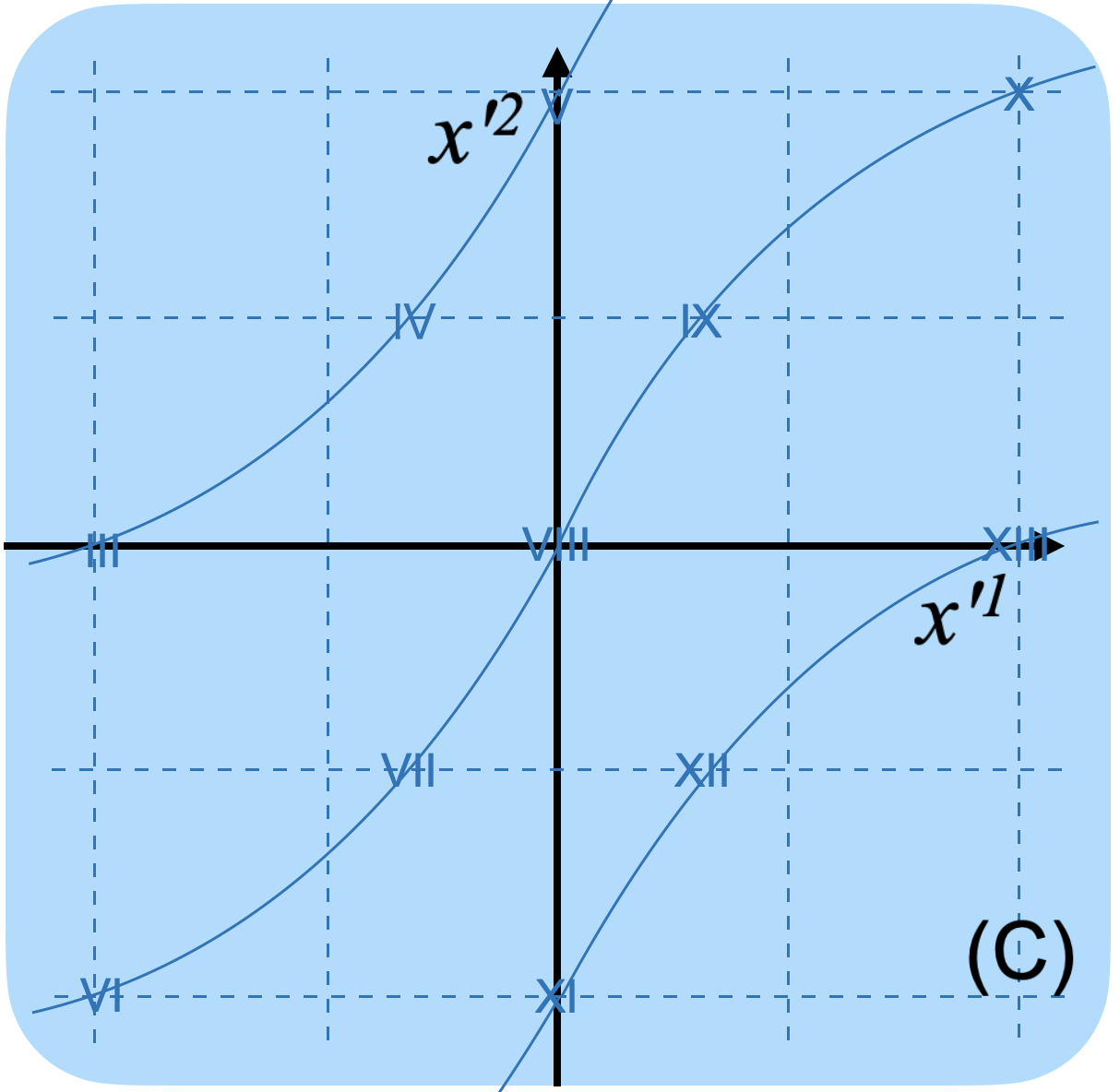
Therefore, this transformation qualifies as a diffeomorphism. The ability to establish a second coordinate
system through such a diffeomorphic transition function is the defining condition for whether an
object is a manifold.
2.6.11.2.3.5 Equivalent Transformation of Manifolds
2.6.11.2.3.5.1 General Theory of the Equivalent Transformation of Manifolds
In this section, the general theory of the Equivalent Transformation of Manifolds is explained. Here, "equivalence" refers to either homeomorphism or diffeomorphism.
While these concepts were previously introduced to define the nature of manifolds, they are employed here again to clarify the underlying structure (the "edifice") of how manifolds transform.
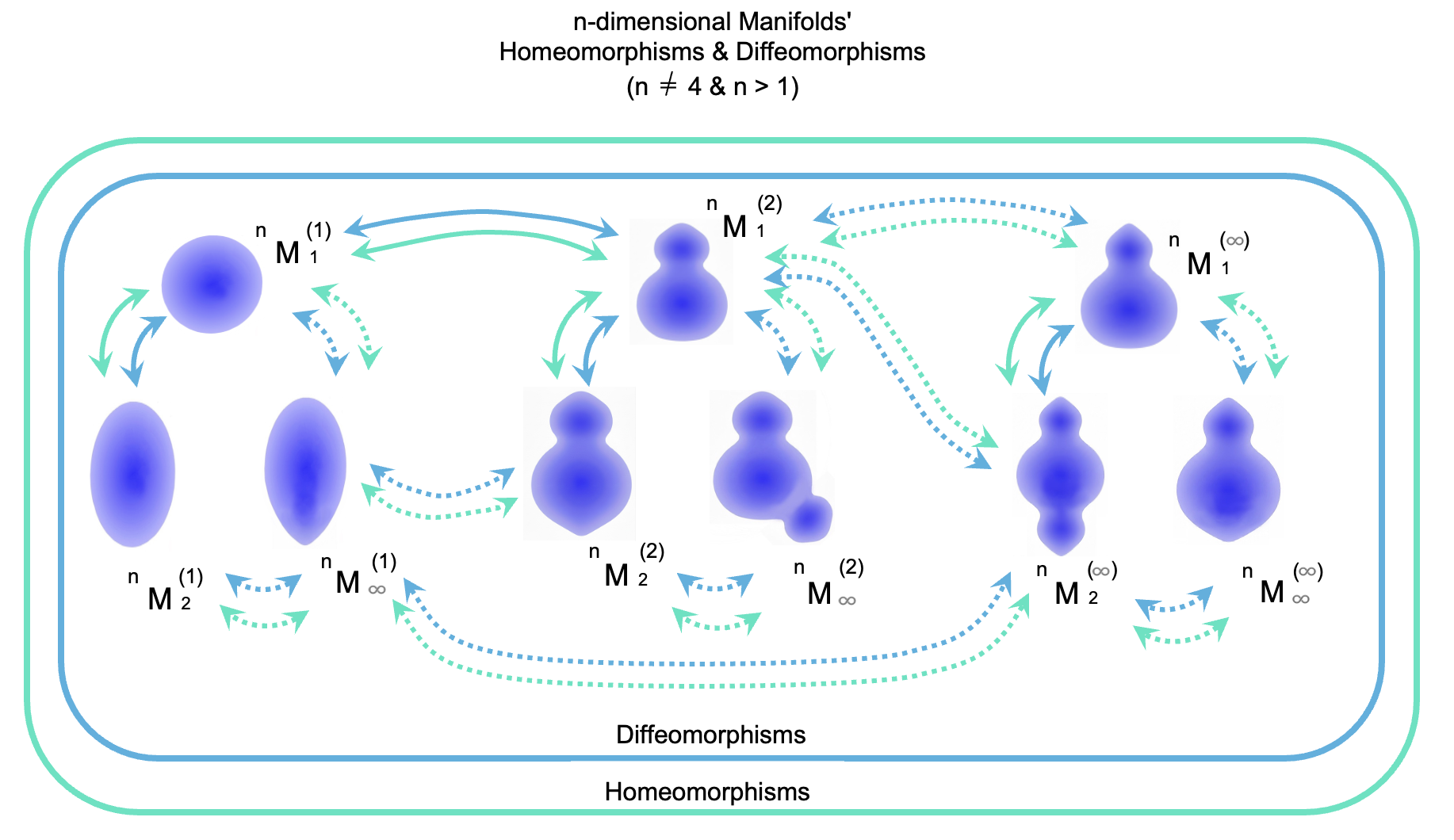
The diagram below illustrates how manifolds evolve through equivalent transformations. For clarity, these manifolds are represented as $n$-dimensional, where $n$ is a natural number greater than 1 ($n > 1$). Although the illustrations may resemble 2-dimensional shapes, they serve as conceptual representations for manifolds of any dimension, as 3-dimensional or 4-dimensional structures are difficult to visualize on a flat surface.
Each manifold is denoted by the symbol ${}^n M_i^{(j)}$. In this notation:
$M$: Stands for Manifold.
$n$ (upper-left): Denotes the dimension of the manifold.
$i$ (lower-right): A serial number assigned to specific transform operations.
$(j)$ (upper-right): A serial number assigned to a specific group of transform operations.
For any given dimension, the initial manifold is denoted as ${}^n M_1^{(1)}$. A manifold resulting from a specific transform operation is denoted as ${}^n M_2^{(1)}$, the subsequent one as ${}^n M_3^{(1)}$, and a manifold following an infinite sequence of such transformations is represented as ${}^n M_\infty^{(1)}$.
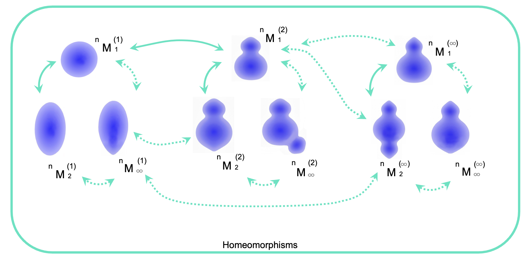
Similarly, starting again from the initial $ {}^n M_1^{(1)} $, a manifold resulting from a different type of transform operation is denoted as $ {}^n M_1^{(2)} $. The manifold after a subsequent transformation of this type is $ {}^n M_2^{(2)} $. Continuing the type of transformation that leads from $ {}^n M_1^{(1)} $ to $ {}^n M_1^{(2)} $ for an infinite number of steps results in the manifold $ {}^n M_1^{(\infty)} $.
All transform operations illustrated in this diagram are homeomorphisms, meaning they preserve topological continuity throughout the transformation. (To maintain focus on the core concepts, we assume here that these transformations do not result in the formation of sharp edges or corners.) In this manner, homeomorphisms can be performed for each dimension, allowing for the transformation of manifolds into virtually any shape.
Furthermore, in almost all dimensions (where $n \neq 4$), these transformations simultaneously satisfy the conditions of a diffeomorphism. This implies that in these dimensions, any manifold reached through a homeomorphism can also be mutually reached through an infinitely differentiable transformation. Consequently, for a given topological shape, there exists only one unique differentiable structure. In other words, all such manifolds belong to a single, unified group (differentiable structure) under diffeomorphism.
The condition that a homeomorphism necessarily implies a diffeomorphism has been rigorously proven over the course of the 20th century:
For 2-dimensional manifolds: This was proven in the early 20th century by mathematicians such as Tibór Radó.
For 3-dimensional manifolds: The proof was established in the 1950s by Edwin Moise.
For manifolds of dimension 5 and higher: In the 1960s, Stephen Smale’s proof of
the "Generalized Poincaré Conjecture" utilized the h-cobordism theorem, which revealed
that the variations of differentiable structures are limited to a finite number.
Furthermore, during the 1960s, John Stallings and others proved that for Euclidean
spaces specifically, there exists only one unique differentiable structure in
dimensions 5 and higher.
In the previous sections, 1-dimensional manifolds were not explicitly mentioned.
This is because their appearance—typically represented as a circle or a rubber band—is so distinct from the 2-dimensional or higher manifolds illustrated above, and it might cause confusion if 1-dimensional manifolds are mentioned together.
However, as shown in the diagram below, a 1-dimensional manifold can be visualized
quite simply. Despite the difference in appearance, the fundamental property remains
the same: a homeomorphism also necessarily implies a diffeomorphism. This fact was
established around 1910 CE by the mathematician L.E.J. Brouwer.

2.6.11.2.3.5.2 The Equivalent Transformation of 4-Dimensional Manifolds
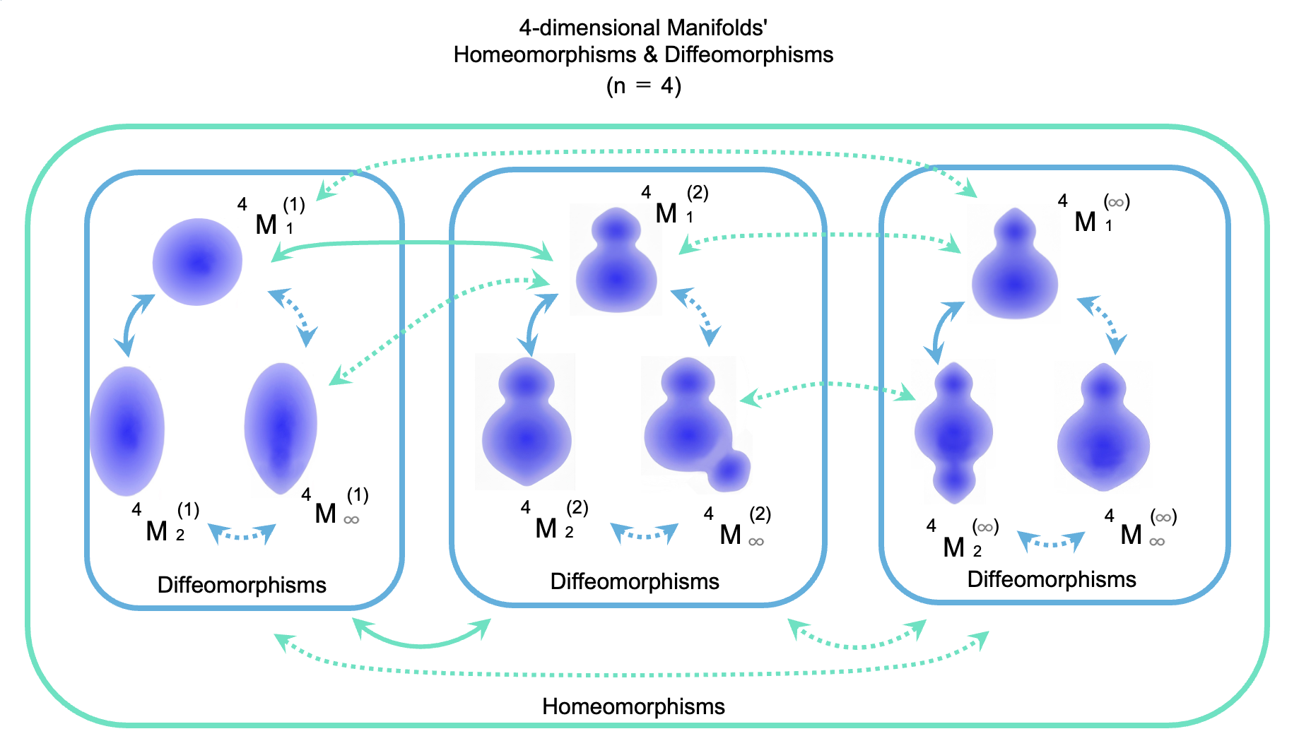
While the relationships described previously hold for almost all dimensions, the situation is fundamentally different for 4-dimensional manifolds. Donaldson's Theorem, discovered in 1982 CE, originally concerned 4-dimensional Euclidean space. However, because Euclidean spaces and manifolds share similar properties, the implications of Donaldson's Theorem extend to 4-dimensional manifolds as well. It has been revealed that the conventional relationship between homeomorphisms and diffeomorphisms does not hold in the 4-dimensional case.
In 4-dimensional manifolds, one can still perform continuous homeomorphisms to create manifolds of virtually any shape. However, in these transformations, a diffeomorphism is almost never satisfied. The specific situation is illustrated in the diagram below.
In this diagram, the initial manifold is denoted as $ {}^4 M_1^{(1)} $. A manifold resulting from a single deformation that satisfies the conditions of a diffeomorphism is $ {}^4 M_2^{(1)} $. Subsequent manifolds following further diffeomorphic deformations are denoted as $ {}^4 M_3^{(1)} $, and after an infinite number of such deformations, the manifold is denoted as $ {}^4 M_\infty^{(1)} $.
Starting again from the initial $ {}^4 M_1^{(1)} $, a manifold resulting from a single homeomorphism (which is not a diffeomorphism) is denoted as $ {}^4 M_1^{(2)} $. From this point, a manifold resulting from a subsequent diffeomorphic deformation is denoted as $ {}^4 M_2^{(2)} $. Furthermore, the result of infinite homeomorphisms starting from $ {}^4 M_1^{(1)} $ toward a different structure is denoted as $ {}^4 M_1^{(\infty)} $.
In 4-dimensional manifolds, while any shape can be created through homeomorphisms, a diffeomorphic relationship exists only among manifolds that have been transformed from the original via diffeomorphic transformations. In other words, in 4D, manifolds related by diffeomorphic transformations form a single distinct group known as a Differentiable Structure.
Manifolds that are related only by a simple homeomorphism belong to different groups. Consequently, there exist many—in fact, infinitely many—distinct groups (differentiable structures) that are homeomorphically equivalent but diffeomorphically distinct. This phenomenon is described as the existence of infinite Exotic Differentiable Structures in 4-dimensional manifolds. This includes 4-dimensional Euclidean space itself.
2.6.11.2.4 The Emergence of Two Major Trends around 1985 CE
2.6.11.2.4.1 Outline
Regarding the unification of gravitational theory and quantum mechanics, it can be said that the two major trends in modern physics, which have continued for the subsequent 40 years, began around 1985 CE.
While there are no official names for these two major trends, they may be designated as follows:
(a) Background-Dependent Continuum Holography School
(b) Background-Independent Discrete Network School
(a) Background-Dependent Continuum Holography School
This school operates on the premise that the universe and its complex structures already exist. It seeks to explain the mechanisms of the universe without necessarily questioning the fundamental reason for its existence. (However, a limitation of this theory is perceived in its failure to delve into why the universe and its complex structures came to be.) This school begins with the assumption that space is a smooth continuum and posits the existence of short strings as a concept to replace conventional elementary particles.
(b) Background-Independent Discrete Network School
This school investigates the reasons behind the existence and the formation of the complex structures of the universe. It considers spacetime to be a discrete network formed by the interconnection of fundamental minimum units, rather than a smooth continuum.
2.6.11.2.4.2 Green and Schwarz’s Superstring Theory in 1984 CE
2.6.11.2.4.2.1 Background
This theory (Superstring Theory) belongs to the (a) Background-Dependent Continuum Holography School.
In the unification of gravitational theory and quantum mechanics, the conventional standpoint of treating particles as "points" leads to the problem of Infinite Divergence (or Ultraviolet Divergence). This occurs because the force becomes infinite when the distance between particles reaches zero. According to Newton’s law of universal gravitation, if the distance $r$ between two particles is zero, the denominator becomes zero, rendering further calculation impossible.
According to Newton’s law of universal gravitation, if the distance $r$ between two particles is zero, the denominator becomes zero, rendering further calculation impossible.
$F = G \frac{m_1 m_2}{r^2}$
$F$: Strength of Gravity
$r$: Distance between two particles
If a particle is a "dimensionless point," the distance $r$ becomes zero when two particles perfectly overlap.
To address this, a theory emerged proposing that what have conventionally been called "particles" are actually "short strings." However, this early string theory (known as Bosonic String Theory) faced the following challenges:
It could only represent bosons (force-carrying particles).
It could not represent fermions (matter particles).
It predicted the existence of mysterious particles called "tachyons."
For massless particles like photons (a type of boson) to exist, the theory required 25 dimensions of space (26 dimensions of spacetime).
Meanwhile, the theory of "Supersymmetry," which posits a symmetry between bosons and fermions, had been proposed by Howard Georgi and Savas Dimopoulos.
2.6.11.2.4.2.2 Superstring Theory
In 1981 CE, Michael Green and John Schwarz proposed Superstring Theory, which introduced supersymmetry into string theory. Following intensive study through 1985 CE, it was confirmed that Superstring Theory possessed several superior characteristics:
Fermions (matter particles) could be represented.
Tachyons were eliminated.
Ten dimensions of spacetime were sufficient (9 dimensions of space + 1 dimension of time).
Superstring Theory likens various particles to tiny, vibrating strings. It attempts to explain diverse particles, forces, and other phenomena through these microscopic strings. Different vibration modes represent different quantum properties. The length of a string corresponds to the Planck length ($1.616 \times 10^{-35}$ meters).
There are several variations of Superstring Theory regarding specific details. The initial version by Green and Schwarz (Type I) assumed the existence of both "closed strings" (loops) and "open strings" (standard strings without loops). According to Type I Superstring Theory, closed strings correspond to gravitons, while open strings correspond to other elementary particles. Subsequently, several other versions of Superstring Theory were proposed.

However, even though the requirement was reduced from 26 dimensions, the theory still necessitated 10 dimensions of spacetime. This left the significant problem of how to interpret the existence of six extra dimensions of space beyond the three dimensions of familiar space.
*By the way it should be noted that "Strings" or "Superstrings"
would be a parable to
explain the properties of particles (or waves).
*In addition, it should be noted that "Strings" or "Superstrings" is
presumed vibrating, and moreover, dominated by the Uncertainty Principle.
*Aside from that, it should be noted that Superstring Theory
wouldn't be associated with the General Theory of Relativity.
Superstring Theory yet has no proper theory on Gravity.
*In short, Superstring Theory is incorrect.
Yet, its multiverse theory (mentioned below) is instructive and
attempt to unify a considerable number of elementary particles is agreeable.
*
"Superstring Theory in Wikipedia"
http://en.wikipedia.org/wiki/Superstring_theory
*
"SUPERSTRING!"
http://www.sukidog.com/jpierre/strings/index.html
*
"String Theory Website Basics"
http://www.superstringtheory.com/basics/index.html
*
"First Superstring Revolution in Wikipedia"
http://en.wikipedia.org/wiki/First_superstring_revolution#1984-1989:_first_superstring_revolution
2.6.11.2.4.3 Calabi-Yau Manifolds by Candelas, Horowitz, Strominger, and Witten in 1985 CE
Background:
To maintain the mathematical consistency of Superstring Theory—specifically to eliminate mathematical infinities and contradictions—a significant challenge remained: the theory necessitated six extra spatial dimensions in addition to the existing four-dimensional spacetime (three dimensions of space and one dimension of time).
Calabi-Yau Manifolds:
Candelas and his colleagues introduced "Calabi-Yau manifolds," a mathematical geometric structure, to account for the unobservable six extra dimensions. According to this theoretical assumption, these extra dimensions are "compactified" (curled up) into an infinitesimal region at the Planck scale.
Diversity and Difficulties:
It is estimated that there are more than $10^{500}$ possible configurations for the shape of Calabi-Yau manifolds and the patterns of energy distribution (the landscape) wrapped around them. This diversity stems from the complex structure of "holes" within the manifolds. Given this vast number of possibilities, it has proven difficult to provide a logical explanation for why our specific universe came to possess its particular set of physical constants out of so many possibilities. (The Landscape Problem)
*
"Calabi-Yau Manifold in Wikipedia"
http://en.wikipedia.org/wiki/Calabi%E2%80%93Yau_manifold
*
"Universe-Review Calabi-Yau"
http://universe-review.ca/R15-26-CalabiYau.htm
2.6.11.2.4.4 Ashtekar Variables in 1986 CE
It can be said that the (b) Background-Independent Discrete Network School originated with the introduction of Ashtekar variables in 1986 CE. While Einstein's field equations represent the curvature of spacetime, combining them with quantum theory proved extremely difficult for computation.
Under these circumstances, Abhay Ashtekar devised a method to reformulate the curvature of space into a format different from Einstein's original equations. This reformulation is known as Ashtekar variables.
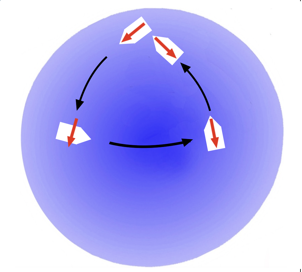
Ashtekar focused his work on three-dimensional space, conceptualizing a vast number of small loops within it. Within a given loop, a vector (indicated by an arrow) is assumed to point in a specific direction from a starting point. As continuous movement occurs along the loop, any curvature in the path is reflected in the orientation of the vector. The vector is adjusted so that it always points in a direction that compensates for the turn. Upon completing a full circuit of the loop, the vector will point in the same direction as it did at the start if the space is flat.
For example, in two-dimensional space, performing this on a flat plane results in the vector pointing in the original direction upon return. (Even on a surface like a cylinder, the vector orientation remains unchanged.) However, in the case of a loop placed on a spherical surface, the direction at the start and the finish will differ.
While the term "loop" is used here, it may be easier to visualize these as polygons rather than perfect circles. Since the same logic applies to paths consisting of straight lines and right-angle turns, the following explanation utilizes an example of a vessel moving in straight lines with 90-degree turns.
Example 1: Movement on a Flat Surface
Assume a flat sea. A vessel starts at a given point, with a red arrow indicating South. The vessel then proceeds South, with the red arrow pointing in the direction of travel. After traveling a certain distance, the course is changed to the East. Since this involves a 90-degree left turn, the red arrow is adjusted to point to the vessel's right. After traveling the same distance, the course is changed to the North. Again, following a 90-degree left turn, the red arrow is adjusted to point toward the vessel's stern (rear). After another equal distance, the course is changed to the West. With a final 90-degree left turn, the red arrow points to the vessel's left. Upon returning to the starting point, the red arrow points in the exact same direction as it did at the departure. This is because there was no distortion (curvature) in the sea.

Example 2: Movement on a Spherical Surface
Assume a spherical surface resembling the Earth, where the topmost point is the North Pole (90°N, 0°E). A vessel starts at the North Pole, with a red arrow pointing South along the 0° longitude line. The vessel proceeds South with the red arrow pointing in the direction of travel. At the equator (0°N, 0°E), the course is changed to the East. Following a 90-degree left turn, the red arrow is adjusted to point to the vessel's right. Upon reaching the point at 0°N, 90°E, the course is changed to the North. Following another 90-degree left turn, the red arrow is adjusted to point toward the vessel's stern. Upon sailing North and returning to the North Pole, the red arrow is shifted 90 degrees from its original orientation. This occurs because the path was set on a curved spherical surface. In this manner, the curvature of space can be measured.
By expressing the curvature of three-dimensional space in this way, it became possible to perform calculations that integrate the curvature of space with quantum theory.
*
"Ashtekar Variables on Wikipedia"
https://en.wikipedia.org/wiki/Ashtekar_variables
2.6.11.2.5 Eternal Inflation by Linde in 1986 CE
Background:
Alan Guth attempted to explain cosmic inflation through the "quantum tunneling effect," assuming a state of "false vacuum." However, such a one-time-only theory was considered insufficient as a comprehensive outlook on the nature of the cosmos.
Linde’s Eternal Inflation:
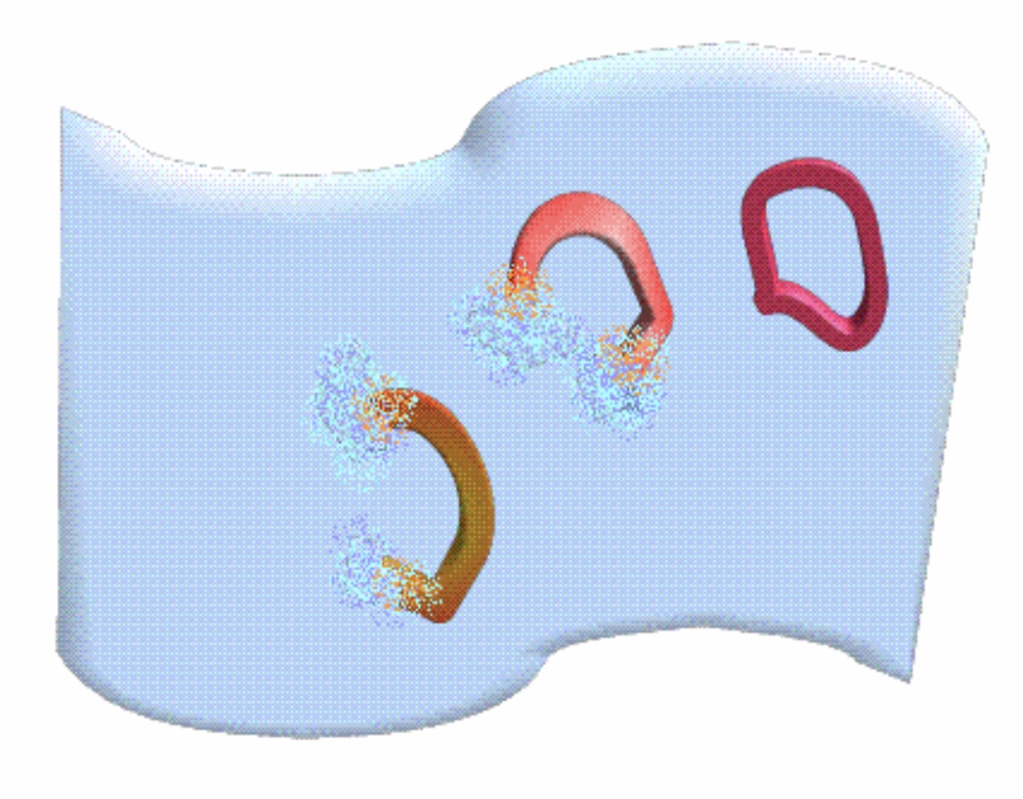
Andrei Linde proposed that the "Mother Universe" continues to expand eternally. Within this vast expansion, "baby universes" are generated randomly (chaotically), much like bubbles forming in carbonated water or cracks appearing in a medium. Each baby universe initiates its own inflationary expansion. This model was designated as "Chaotic Inflation."
In this theory, space is treated as a "smoothly expanding fluid" (a scalar field). Spacetime is calculated not as a collection of a vast number of discrete components, but as a continuum—resembling a rubber membrane that can be stretched indefinitely. Furthermore, this theory does not provide an explanation for its own ultimate origin.
*
"Eternal Inflation on Wikipedia"
http://en.wikipedia.org/wiki/Eternal_inflation
*The random creation of the baby universes in the
eternal inflating Mother Universe would be depicted as follows.

Consequently, this model can be classified under the lineage of the (a) Background-Dependent Continuum Holography School.
2.6.11.2.6 Weinberg’s Multiverse and the Anthropic Principle in 1987 CE
Background:
Based on the hypothesis of "spacetime continuity," the pursuit of mathematical consistency led to Superstring Theory—dealing with ten-dimensional spacetime—emerging as the unique solution. However, this necessitated an explanation (or justification) for the "six extra dimensions," leading to the introduction of the concept of infinitesimally curled-up "Calabi-Yau manifolds." It is estimated that there are approximately $10^{500}$ different configurations of Calabi-Yau manifolds. Meanwhile, research into the fundamental constants of physics continued to progress.
Weinberg’s Multiverse and the Anthropic Principle:
Steven Weinberg noted that various fundamental constants appear to be extremely finely tuned to values favorable for the existence of life.
Regarding the "flatness problem," the critical density required for the universe to exist stably after the Big Bang—without either collapsing or expanding excessively—is approximately $10^{-26} \text{ kg/m}^3$ (expressed as energy density converted to mass). Based on observation technology in 1987 CE, the observed density of the universe was considered to be almost consistent with this value.
In stark contrast, the Planck density derived from quantum theoretical inferences (the calculation of vacuum energy) is $5.1 \times 10^{96} \text{ kg/m}^3$. In other words, the observed density of the universe is approximately 120 orders of magnitude smaller than the theoretical "vacuum density." Explaining this immense discrepancy between the theoretical vacuum and the energy density of the actual universe presents a significant problem.
On the other hand, standard theories suggest that $10^{500}$ or more configurations of Calabi-Yau manifolds exist. Weinberg assumed that a single universe is homogeneous as well as continuous, and therefore, a single universe corresponds to one specific type of Calabi-Yau manifold. He argued that in addition to our universe, a vast number ($10^{500}$) of other universes exist, many of which possess unsuitable fundamental constants and are devoid of life. By introducing the concept of spatial homogeneity, it is argued that our universe, with its harmonized fundamental constants, is merely one accidental occurrence among countless others.
Conclusion:
Following the premise that spacetime is continuous, Superstring Theory with ten-dimensional spacetime was identified as the only solution. This necessitated an explanation for the additional six dimensions, provided by the concept of Calabi-Yau manifolds. These extra spatial dimensions are curled up into microscopic Calabi-Yau manifolds. However, since there are $10^{500}$ types of Calabi-Yau configurations, and assuming that spacetime within a single universe must be homogeneous, each universe must consist of only one specific configuration.
This led to the hypothesis of an infinite number of universes ($10^{500}$ types), each with different Calabi-Yau manifolds. In our particular universe, a miraculous accident occurred, resulting in a stable universe with a density and fundamental constants capable of supporting life, far removed from the Planck density. This is the explanation provided by the Anthropic Principle: humans exist because such an accident occurred.
*
"Flatness Problem in Wikipedia"
http://en.wikipedia.org/wiki/Flatness_problem
*
Planck Density in Wikipedia"
http://en.wikipedia.org/wiki/Planck_density
*
"Anthropic Principle in Wikipedia"
http://en.wikipedia.org/wiki/Anthropic_principle
Unsurprisingly, this theory belongs to the (a) Background-Dependent Continuum Holography School.
2.6.11.2.7 The $\Lambda$-CDM Model by COBE in 1992 CE
Background:
Albert Einstein originally introduced the cosmological constant ($\Lambda$) as a "repulsive force" acting against gravity to maintain a static universe. This is represented in the Einstein field equations as follows:
$G_{\mu\nu} + \Lambda g_{\mu\nu} = \frac{8\pi G}{c^4} T_{\mu\nu}$
Left side ($G_{\mu\nu} + \Lambda g_{\mu\nu}$): The geometry and curvature of spacetime.
Right side ($T_{\mu\nu}$): The distribution of matter and energy.
The $\Lambda$-CDM Model:
In 1989 CE, NASA launched the COBE (Cosmic Background Explorer) satellite, which conducted precise observations of the Cosmic Microwave Background (CMB) radiation. These observations led to the discovery of "fine-scale temperature anisotropies (fluctuations)" in the CMB. These fluctuations served as the "seeds" that allowed matter to clump together and form stars and galaxies. Through simulations of this formation process, it was concluded that the gravity provided by ordinary matter alone was insufficient, necessitating the presence of a vast amount of Cold Dark Matter (CDM).
As a result, the standard model of modern cosmology, known as the "$\Lambda$-CDM model," was established. This model reintegrates the cosmological constant ($\Lambda$) into Einstein's gravitational equations and combines it with CDM. While Einstein originally introduced $\Lambda$ with a static universe in mind, modern cosmology defines $\Lambda$ as "dark energy," the force responsible for accelerating the expansion of the universe.
*
"Cosmic Background Explorer in Wikipedia"
http://en.wikipedia.org/wiki/Cosmic_Background_Explorer
*
"Lambda-CDM Model in Wikipedia"
http://en.wikipedia.org/wiki/Lambda-CDM_model
2.6.11.2.8 Loop Quantum Gravity by Smolin in 1994 CE
2.6.11.2.8.1 Background:
To a certain extent, Superstring Theory has succeeded in explaining the Standard Model, the "three forces," and mass. However, Superstring Theory does not explicitly address "space (distance)" or "time" itself. This implies a weak connection with General Relativity, which concerns gravity.
As previously mentioned, Einstein asserted in the General Theory of Relativity that there is an intimate relationship between gravity, space, time, and the curvature of spacetime. Rather, he argued that gravity is not a "force" but the very property of "curved spacetime." To unify the General Theory of Relativity (including gravity) with quantum theory, the curvature of spacetime itself must be taken into account.
The invention of Ashtekar variables by Abhay Ashtekar—which reformulated the General Theory of Relativity into a format utilizing "loops" within space—enabled calculations between the General Theory of Relativity and quantum theory.
2.6.11.2.8.2 Loop Quantum Gravity:
The Standard Model (including Superstring Theory) treats gravity as "particles (gravitons) flying over a background spacetime." In contrast, Loop Quantum Gravity (LQG) and the subsequently described Spin Foam theory posit, based on General Relativity, that the "distortion of the spacetime network itself" is the true nature of gravity.
LQG describes the minimum units of space geometrically as polyhedra, such as cubes, with sizes on the order of the Planck length ($1.616 \times 10^{-35}$ meters). These are simplified into "nodes" and "lines" (edges).
Rather than having pre-existing shapes for these minimum units of space, the "connectivity" of the network determines the shape of the spatial units. This theory is predicated on the existence of a "minimum unit of spacetime."
As an example, consider a cube with sides of two Planck lengths (used here as a hypothetical assumption for explanation). The center point of this three-dimensional shape is defined as a "node," generally represented as a point. This node corresponds to the "volume" possessed by the minimum unit of space. In LQG, space itself is quantized (existing in states represented by simple integers of the fundamental units), and each node is assigned a label of quantum information called "spin."

From the node, lines (edges) extend through the center of each face of the cube (squares) to connect with adjacent minimum units of space. These nodes represent "volume," while the extending lines represent "area" (furthermore, specific numerical data, such as volume = 8 or area = 4, are assigned as data). Consequently, three-dimensional shapes like cubes are simplified into a network of nodes and lines.
When other shapes, such as square pyramids, are added, they are depicted similarly.
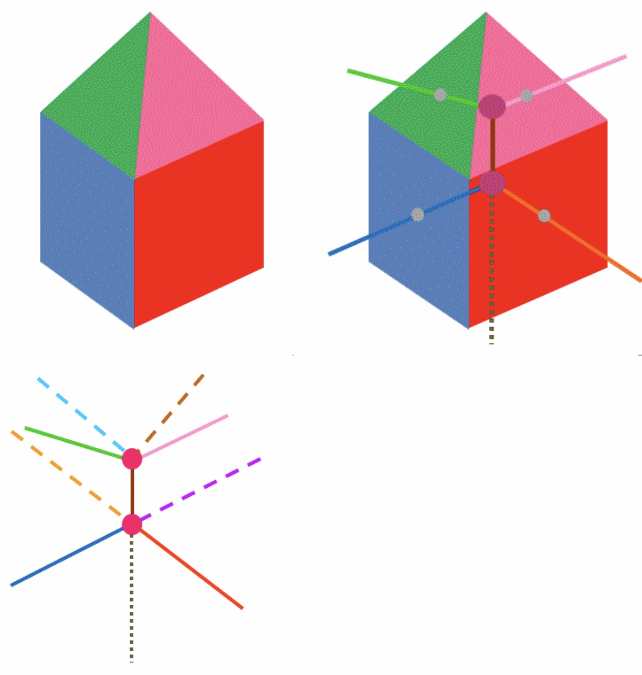
LQG assumes that space is filled with these nodes (representing quanta of spatial volume) and the lines connecting them (representing quanta of spatial area). These are called "Spin Networks."
Tracing the lines (edges) within this network reveals that they connect to each other without interruption, forming closed "loops." This is the origin of the term "Loop" in the theory's name, and the overlapping of these countless loops is the true identity of what is called "space." Curved space is represented by the patterns of these network connections (their density and distortion). These loops are not merely a mesh; they also serve as indicators for measuring the curvature of space. Using the method of Ashtekar variables, the curvature of space can be measured in a manner compatible with the General Theory of Relativity.
*
"Universe Review Quantum Gravity"
http://universe-review.ca/R01-07-quantumfoam.htm
*
"Loop Quantum Gravity Einstein Online"
http://www.einstein-online.info/elementary/quantum/loops
*
"Loop Quantum Gravity in Wikipedia"
http://en.wikipedia.org/wiki/Loop_quantum_gravity
2.6.11.2.9 Proposal of Spin Foam around 1997 CE
2.6.11.2.9.1 Background
The "Spin Networks" proposed by Lee Smolin and others in 1994 CE successfully provided a quantum description of the "structure of space" at a given moment. However, to achieve a complete quantization of gravity, it was necessary to incorporate the "passage of time (the evolution of spacetime)" as demonstrated by Einstein’s General Theory of Relativity.
2.6.11.2.9.2 Spin Foam
Carlo Rovelli, John Baez, and others proposed the "Spin Foam" theory, which describes the process of spin networks evolving over time as a geometric structure resembling overlapping bubbles (foam). When a "line" in a spin network moves through time, it sweeps out a "surface"; similarly, when an "intersection (node)" moves, it traces a "line." This established a framework for performing quantum mechanical calculations not only for static space but for four-dimensional spacetime itself.
For instance, suppose three nodes and the three lines connecting them form a triangle (as part of a spin network). If that triangle does not move over time, its progression through time is depicted as a triangular prism. (Note: While Spin Foam is often depicted with time progressing downwards, the following figure of a stationary triangle depicts time progressing upwards, similar to Minkowski spacetime.)
If the three nodes move away from each other over time (or if space curves accordingly), the progression of that triangle through time is depicted as, for example, an inverted square pyramid, an inverted triangular tower, or an inverted trapezoid. Such a representation of the passage of time for a spin network is called a "Spin Foam."

However, it is important to note that the changes in the spin network (e.g., the triangle) are not depicted continuously over time. The triangle is depicted discretely and digitally, like sequential photographs (stroboscopic photography), at intervals such as the Planck time ($10^{-43}$ seconds). Just as television or film images appear to change smoothly but are actually a collection of frequently replaced still images, the transitions of triangles and spin networks (Spin Foam) function in exactly the same way.
*
"Spin Foam on Wikipedia"
https://en.wikipedia.org/wiki/Spin_foam
2.6.11.2.10 Witten's M-Theory in 1995 CE
Background
Various Superstring Theories were presented after Type I.
The circumstances became confusing.
Witten's M-Theory
Witten claimed some Superstring Theories would be united employing
11-dimensional Spacetime, instead of 10 dimensional Spacetime,
to be a theory named M-Theory.
*
"M-Theory in Wikipedia"
http://en.wikipedia.org/wiki/M-theory
2.6.11.2.11 Polchinski's D-Branes in 1995 CE
Background
Superstring Theory had to account for extra 6 dimensions.
As mentioned above, an account was Calabi-Yau Manifold.
D-Branes
Polchinski claimed another account of the extra 6 dimensions.
Polchinski claimed high-dimensional objects, named D-Branes.
Some endpoints of Superstrings are connected to D-Branes.
D-Brane was assumed drifting in higher dimensional space.
*For example, a D-Brane would be 3-dimensional space drifting
in 9-demensional space.
The D-Brane of 3-dimensional space represents this universe.
Since the whole space is 9-dimensional,
it amounts to 10-dimensional Spacetime and
Superstring Theory wouldn't fall.
Since this universe is 3-dimensional, the extra 6 dimension wouldn't be realized.
Most Superstrings adhere to Branes.
However, Superstrings of Graviton (closed strings) wouldn't adhere to
Branes and they would rather escape to the extra dimensions.
Then Gravity is extraodinary weaker compared with
other forces ("Hierarchy Problem about Forces").
*This is the excuse by D-Branes Theory.
*
"SUPERSTRINGS! D-Branes"
http://www.sukidog.com/jpierre/strings/dbranes.htm
*
"D-Brane in Wikipedia"
http://en.wikipedia.org/wiki/D-brane
*However, if Gravitons escape to the extra dimensions,
it results in an error that
Gravity wouldn't comply with the Inverse-Square Law.
*
"Inverse-Square Law in Wikipedia"
http://en.wikipedia.org/wiki/Inverse-square_law
*Since dozens of elementary particles couldn't be fundamental existence,
particles should be summarized by appropriate theories such as Superstring Theories.
However, despite such attempts involving Superstring Theories,
Superstring Theories seem drifting and
reaching a dead end without promising
perspectives and
without considering
curvature of Spacetime, the General Theory of Relativity.
Consequently, Superstring Theories would be incorrect.
Yet, some claims of Superstring Theories could be still implicative.
2.6.11.2.12 Riess' Discovery of Accelerating Expansion of the Universe and Dark Energy in 1998 CE
Background
Rubin discovered Dark Matter in the universe amounting to some
10 times than the observable mass.
The observation by COBE implied presence of an enormous amount of
Cold Dark Matter (CDM) and an enormous amount of unknown entities
in the universe represented by Lambda (Λ).
Riess' Discovery of Accelerating Expansion of the Universe and Dark Energy
Riess et al discovered an Acceleration Expansion of the universe.
It implied presence of a hypothetical form of energy amounting to
73-74% of the total mass-energy of the universe.
Subsequently, other observations followed.
The energy was named "Dark Energy."
The Dark Energy might be identified with "Vacuum Energy,"
while details are unknown.
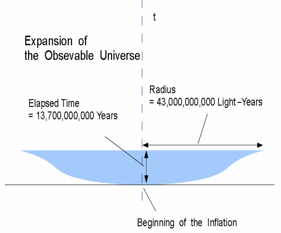
On the other hand, Accelerating Expansion of the Observable Universe
after the Inflation coud be illustrated as follows.
If the observation is correct,
the Whole Universe would be larger than that
(for example 5 times larger in length), but details are unknown.
*
"Observational Evidence from Supernovae"
http://arxiv.org/abs/astro-ph/9805201
*
"Accelerating Universe in Wikipedia"
http://en.m.wikipedia.org/wiki/Accelerating_universe
*
"Dark Energy in Wikipedia"
http://en.wikipedia.org/wiki/Dark_energy
*
"Vacuum Energy in Wikipedia"
http://en.wikipedia.org/wiki/Vacuum_energy
2.6.11.2.13 Zeilinger' Verification of Quantum Entanglement in 1999 CE
Zeilinger verified Quantum Entanglement on photons.
It means 2 waves (particles) are related regardless of distance and
Nonlocality in this Universe.
*
"Anton Zeilinger in Wikipedia"
http://en.wikipedia.org/wiki/Anton_Zeilinger
*
"Science News 75 Years of Entanglement"
https://www.sciencenews.org/article/75-years-entanglement
2.6.11.2.14 Randall and Sundrum's Warped Extra Dimensions in 1999 CE
Background
As mentioned above, if D-Branes Theory claims that Gravitons escape to the extra dimensions,
it results in an error that Gravity wouldn't comply with the Inverse-Square Law.
Randall and Sundrum's Warped Extra Dimensions
Randall and Sundrum claimed that the extra dimensions are warped (curved) and Gravitons
rarely escape to the extra dimensions, then Gravity approximately comply with
the Inverse-Square Law.
*It sounds like a mere excuse.
*
"Randall-Sundrum Model in Wikipedia"
http://en.wikipedia.org/wiki/Randall%E2%80%93Sundrum_model
2.6.11.2.15 WMAP's Observation in 2001 CE
Background
NASA's WMAP succeeded COBE.
WMAP's Observation
WMAP's Observation supported presence of an enormous amount of Dark Energy.
Then the universe is presumed consisting of
74% unknown Dark Energy, 22% unknown Dark Matter, and some 4% of ordinary matter.
Other than that, WMAP estimated the radius of the observable universe
to be more than 39 billion light years.
*
"Universe Review"
http://universe-review.ca/F02-cosmicbg.htm
*
"Observable Universe"
http://en.wikipedia.org/wiki/Observable_universe
2.6.11.2.16 Khoury, Ovrut, Steinhardt, and Turok's Ekpyrotic Universe in 2001 CE
Background
The origin of the Big Bang was controversial.
D-Branes Theory was claimed to account for the extra 6 dimension of Superstring Theory.
Ekpyrotic Universe
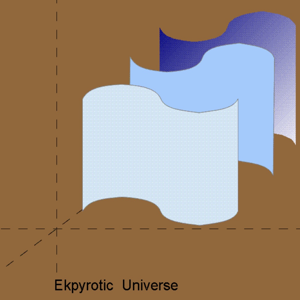
Khoury, Ovrut, Steinhardt, and Turok proposed the Ekpyrotic Universe Theory.
According to the Ekpyrotic Universe Theory,
this 3-dimensional universe and other similar 3-dimensional
universes
are drifting in a higher dimensional Mother Universe.
two of the 3-dimensional universes (baby universes) would sometimes collide.
Then this universe came from
a collision of two 3-dimensional universes.
The 3-dimensional universes are compared to branes (D-Branes).
*
"Ekpyrotic Universe in Wikipedia"
http://en.wikipedia.org/wiki/Ekpyrotic_universe
*3-dimensional spaces (Universes) in the higher dimensional Mother Universe
are compared to 2-dimensional branes like in the following depiction.
*Since a D-Brane corresponds to a universe, the claim of Ekpyrotic Universe Theory
means that a collision of two baby universes (through an extra dimension)
resulted in the Big Bang.
2.6.11.2.17 Susskind's Landscape Theory in 2003 CE
Background
According to Superstring Theory, Calabi-Yau Manifold was an account of the extra 6 dimensions.
Calabi-Yau Manifold has 10^150 through 10^500 kinds in configuration.
In relation to Dark Energy, diversity of Calabi-Yau Manifolds and energy levels were disputed.
Susskind's Anthropic Landscape
Susskind presented the concept of Anthropic Landscape representing diversity of physical constants
involving vacua.
The diverse energy levels on graphs seemed like landscapes of mountain ranges.
The concept also represents myriad universes.
*
"String Theory Landscape in Wikipedia"
http://en.wikipedia.org/wiki/String_theory_landscape
*
"The Anthropic Landscape of String Theory"
http://arxiv.org/abs/hep-th/0302219
2.6.11.2.18 Zeilinger's Quantum Entanglement over 144km in 2007 CE
Zeilinger verified Quantum Entanglement on photons over 144km.
It means waves (particles) of photons are related simultaneously regardless of 144km distance.
Return to the Home Page