Disclaimer: This is Untrue.
2.6.12 Presumption of the Whole Inclusive Theory of Everything 1
2.6.12.1 Overview
The major theories of modern physics, while groundbreaking, appear to have reached a plateau without providing a definitive resolution. It seems that the final piece of the cosmic puzzle remains elusive.
This section explores Causal Dynamical Triangulation (CDT), a compelling theoretical framework that stands as a leading candidate for the next breakthrough.
Additionally, an analysis is provided for the Holographic Universe Theory,
an idea proposed from the standpoint of (a) Background-Dependent Continuum Holography School, which reimagines the very nature of reality as a sophisticated projection of information.
2.56.12.2 Details
2.6.12.2.1 Causal Dynamical Triangulation (CDT) in 2005CE
2.6.12.2.1.1 Background
Loop Quantum Gravity (LQG) achieved significant success in describing the fundamental units of spacetime through the introduction of spin networks and spin foams. However, during the early 2000s CE, a formidable mathematical challenge emerged: reconstructing the "smooth 4-dimensional spacetime" of our daily experience from these microscopic elements.
Mathematically, quantum fluctuations often caused spacetime to collapse into a "chaotic state." Specifically, simulations frequently resulted in universes that were either branched into infinitely thin, thread-like structures or crushed into a single, high-dimensional point. These models failed to derive the stable, four-dimensional geometry necessary for a habitable universe.
In response to this impasse, Causal Dynamical Triangulation (CDT)
was introduced. This approach incorporates a fundamental rule?the fixed direction
of time, or "causality"?into the assembly process. By embedding this causal
structure from the start, the theory enables a stable, four-dimensional universe
to self-organize within computer simulations.
2.6.12.2.1.2 Causal Dynamical Triangulation (CDT)
Loll, Ambj?rn, and Jurkiewicz introduced Causal Dynamical Triangulation (CDT) by relaxing certain symmetries found in Loop Quantum Gravity (LQG). The theory functions by assembling fundamental "pieces" according to established physical laws to construct a model of cosmic space. Conceptually, this process bears a resemblance to building structures with geometric toys like Polydron, where triangular pieces are interconnected to form complex shapes.
Utilizing standard computing environments, such as desktop PCs, CDT enables the virtual assembly of these pieces to simulate models of the expanding observable universe within Minkowski spacetime. (It should be noted, however, that like many academic publications, the exhaustive details of the specific algorithms are not always fully disclosed to the public.)
However, since the universe contains unobservable regions, the absolute accuracy of the reconstructed cosmic structure remains an open question.
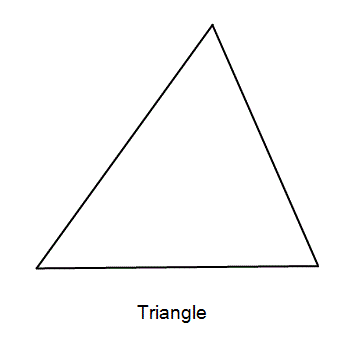
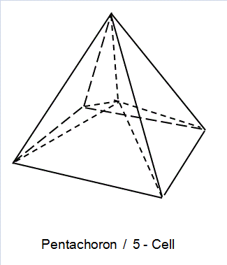
The fundamental components used in CDT are known as simplices (singular: simplex), which are the simplest possible analogues of a triangle in any given dimension. Simplices vary depending on their dimensionality:
2-simplex: A triangle (2nd dimension).
3-simplex: A tetrahedron (3rd dimension).
4-simplex: A pentachoron (also known as a 5-cell), representing the 4th dimension.
In CDT, these simplex "pieces" are assembled via computer simulation to model the spacetime of the universe. Once the properties of the simplices and the governing program are defined, the resulting model is generated through computational processing. Given that the physical universe consists of three
spatial dimensions and one temporal dimension, CDT primarily utilizes
the 4-simplex (pentachoron). However, for the sake of a simplified conceptual
explanation, the following section describes the assembly process using 2D triangular pieces.

*
"Causal Dynamical Triangulation in Wikipedia"
http://en.wikipedia.org/wiki/Causal_dynamical_triangulation
*
"Simplex in Wikipedia"
http://en.wikipedia.org/wiki/Simplex
*
"Scientific American Self Organizing Quantum Universe"
http://www.scientificamerican.com/article.cfm?id=the-self-organizing-quantum-universe
*
"The Emergence of Spacetime or Quantum Gravity on Your Desktop arvix"
http://arxiv.org/abs/0711.0273
*
"Reconstructing the Universe arvix"
http://arxiv.org/abs/hep-th/0505154
2.6.12.2.1.3 Combinations of Triangles
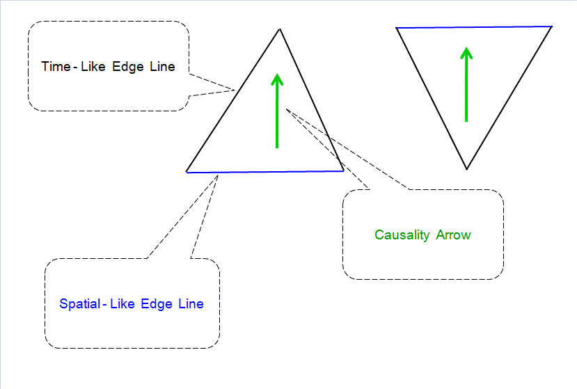
In this conceptual explanation of CDT, a modified triangular model is assumed.
The construction follows specific geometric rules:
(1) grounded in the framework of Minkowski spacetime.
Here, the horizontal axis represents "spatial position," while the vertical axis represents the "passage of time."
(2) Spatial Edges: The horizontal edges of the triangles (indicated in blue) represent spatial dimensions.?
(3) Temporal Edges: The diagonal edges are designated as temporal dimensions.
(4) Causality Arrows: A vertical arrow (indicated in green) is assigned to each triangle to represent causality. Because all physical states evolve over time according to causal laws, this intrinsic directionality is fundamental to the model.
(5) This framework includes both upright triangles and inverted triangles, both sharing the same upward causal orientation.
(6) The physical scale of these pieces is infinitesimally small: the spatial edges are approximately the Planck length ($1.616 \times 10^{-35} \text{ m}$), and the height of each triangle corresponds to the Planck time ($5.39 \times 10^{-44} \text{ sec}$).
(7) Naturally, these triangles must be interconnected at their vertices to maintain structural integrity.
(Note: While some models assume a spatial edge of twice the Planck length to align the diagonal slope with the speed of light [$c = \text{Planck length} / \text{Planck time}$], this explanation follows the standard CDT assumption of "Planck scale." Furthermore, while these triangles are typically equilateral or isosceles in a vacuum, the presence of gravity would warp both the geometry of the triangles and the orientation of the causality arrows.)
*
"Planck Length in Wikipedia"
http://en.wikipedia.org/wiki/Planck_length
*
"Planck Time in Wikipedia"
http://en.wikipedia.org/wiki/Planck_time
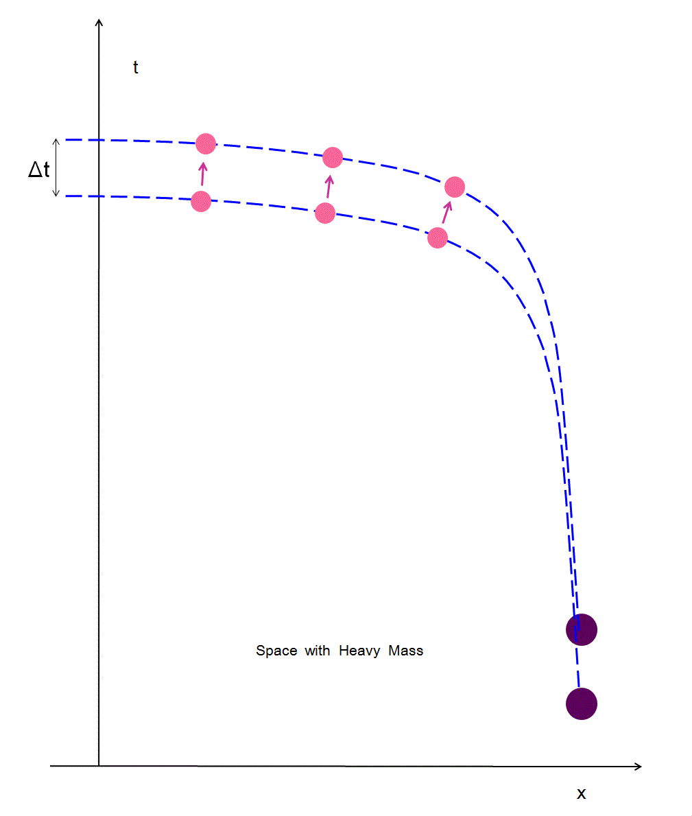
Once these parameters and the governing algorithms are set, the computer begins the process of assembling the triangles to construct a spacetime model. The resulting structure manifests as shown below. The layered regions bounded by the blue spatial lines are known as "Time Slices."
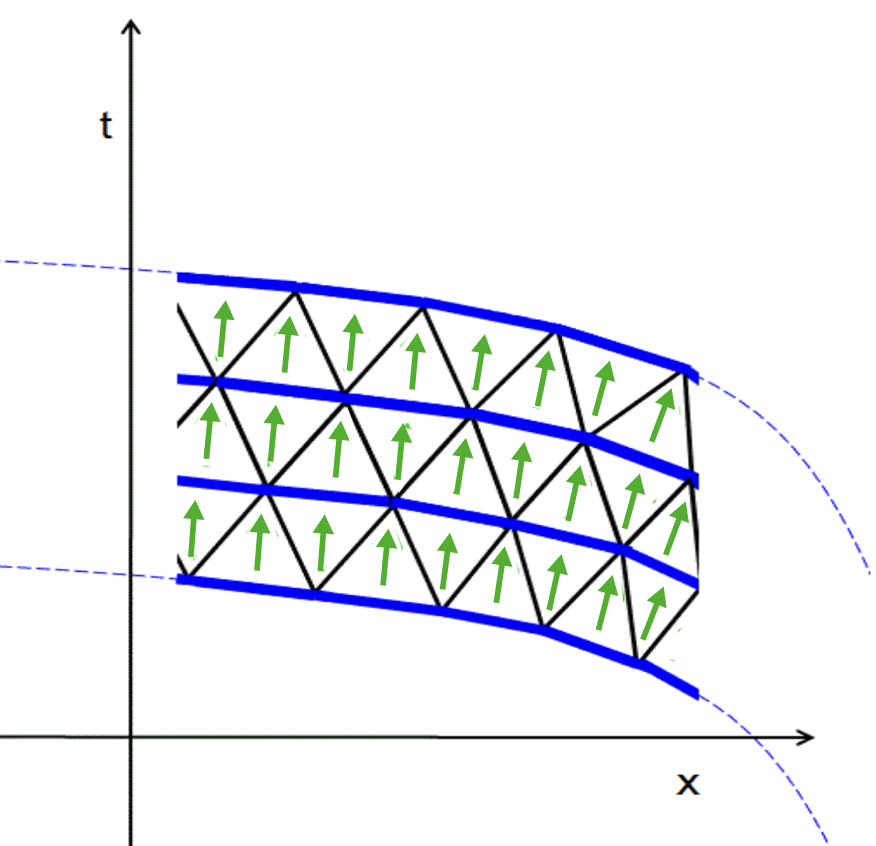
(For reference, the diagram below is fundamentally identical to the one previously presented in the explanation of the General Theory of Relativity.)
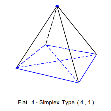
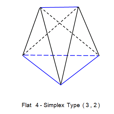
2.6.12.2.1.4 Pentachorons (4-Simplices)
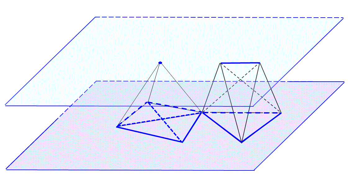
In actual four-dimensional simulations, the pentachoron (a 4-simplex) must be adopted as the fundamental unit. A pentachoron manifests in various forms when projected or sliced within a three-dimensional context.
Two primary examples include the "flat 4-simplex type (4, 1)" and the "flat 4-simplex type (3, 2)."
The following image illustrates how these pentachorons are interconnected across horizontal time slices:
2.6.12.2.1.5 Simulation Results and Dimensionality
2.6.12.2.1.5.1 Introduction of Dimensionality
CDT theory asserts that by introducing specific rules for the "arrows" of
causality (representing the passage of time), a computer can dynamically simulate
a viable spacetime model—one that mirrors the actual spacetime of our universe.
Through the analysis of these simulated models, researchers have calculated their dimensionality.
In the realm of quantum gravity, two distinct concepts of dimension are particularly useful: Hausdorff dimension and Spectral dimension.
Hausdorff Dimension
The Hausdorff dimension is defined as the logarithm of the "scaling of contents" relative to the "scaling of the edges."
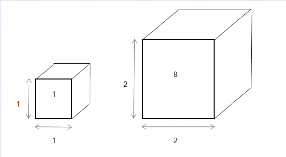
Example (Cube): Consider a cube with an edge length of 1 and a volume (contents) of 1. If the edge length is increased to 2, the volume becomes 8. Since $2^3 = 8$ (i.e., $\log_2 8 = 3$), the Hausdorff dimension of a cube is 3.
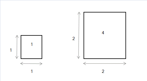
Example (Square): A square with an edge length of 1 has an area (contents) of 1. Increasing the edge length to 2 results in an area of 4. Since $2^2 = 4$ (i.e., $\log_2 4 = 2$), the Hausdorff dimension of a square is 2.
This concept aligns closely with our intuitive understanding of dimensions. However, it can also be applied more abstractly. For instance, in a triangular lattice, if the edge length is extended from a starting vertex, the number of internal triangles (contents) can be counted. If an edge length of 3 contains 5 triangles and an edge of 6 contains 14 triangles, the Hausdorff dimension is expressed as $\log_{6/3} (14/5)$.

Spectral Dimension
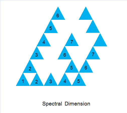
In contrast, the spectral dimension is defined by the logarithm of the "scaling of contents" relative to the "diffusion time." Consider a process starting from a single triangle (No. 1):
At diffusion time $\sigma = 1$, the content is 1 (Triangle No. 1).
At diffusion time $\sigma = 2$, two adjacent triangles are added, totaling 3.
At diffusion time $\sigma = 3$, two more adjacent triangles are added, totaling 5.
At diffusion time $\sigma = 6$, the total content reaches 13.
The "diffusion time" represents the number of steps taken to incorporate adjacent elements, mimicking the physical process of diffusion. In this scenario, the spectral dimension would be $\log_{6/3} (13/5)$.
While similar to the Hausdorff dimension, the spectral dimension is uniquely effective in describing microscopic regions.
The term "diffusion time" is used here not only to observe how a space evolves over time but also to observe how it changes as the measurement scale (magnification) changes.
In domains where measuring distance with a conventional ruler is impossible, "distance" is replaced by "steps of elapsed time."
By observing how an entity spreads over time, one can effectively measure distance and establish a scale for the space itself.
2.6.12.2.1.5.2 Dimensional Reduction
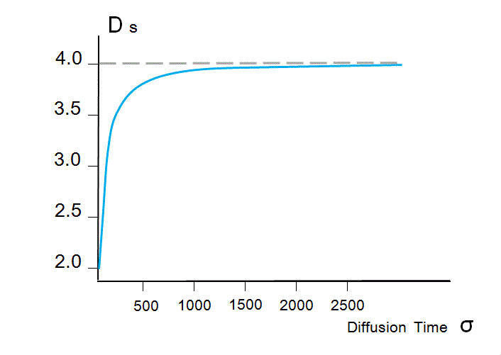
Analysis of the spacetime dimensions simulated via CDT (specifically the spectral dimension) yielded a value of approximately 4.0 at large scales. Given that the simulation primarily utilizes 4-simplices (four-dimensional blocks), this result is expected.
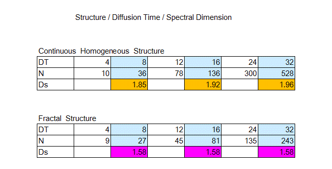
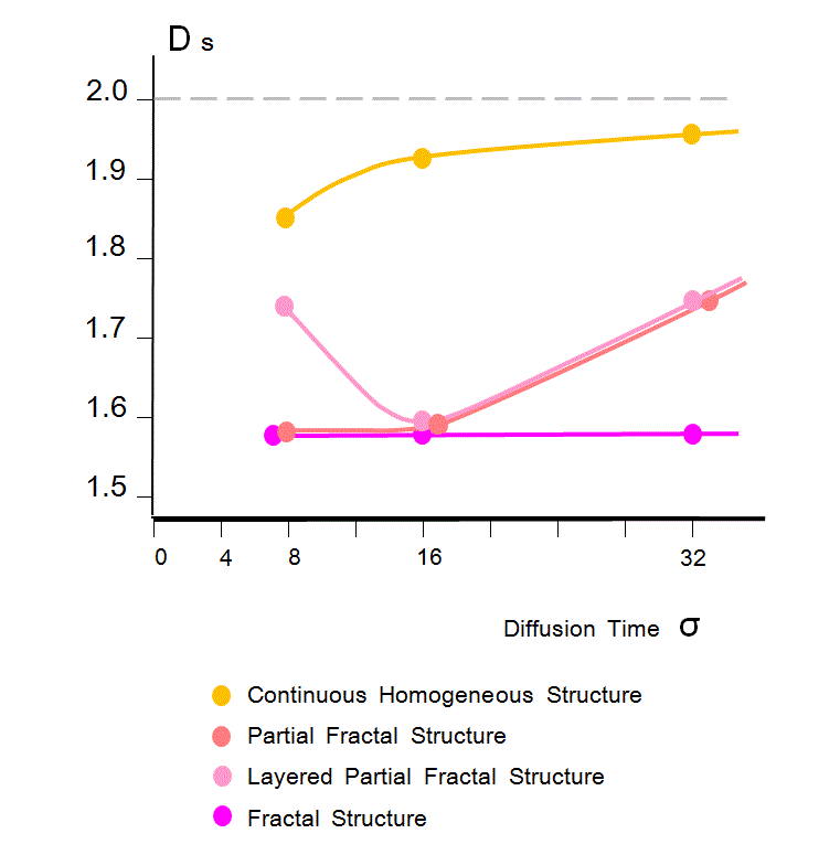
However, a peculiar phenomenon was observed at microscopic scales where both time and distance are infinitesimal. As the diffusion time (the spacetime scale) decreases, the dimensionality of spacetime drops to 2.0. This is illustrated in the diagram below, where $D_s$ represents the spectral dimension:
As established in the definition of the spectral dimension, a reduction in dimensionality implies that as the distance or scale increases, the objects or spaces being counted become increasingly sparse.
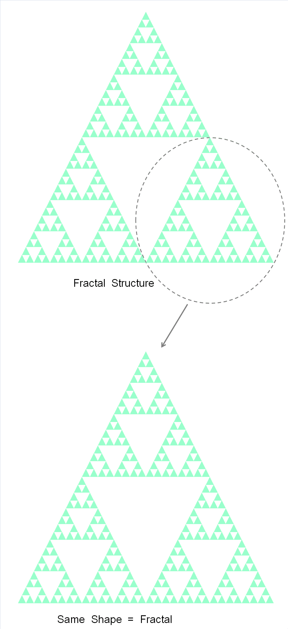
To grasp the essence of this phenomenon, it is insufficient to treat it as a mere statistical anomaly. The underlying principles or rules governing this reduction must be examined. Within CDT, this is interpreted as the spacetime structure transitioning into a fractal structure at microscopic scales.
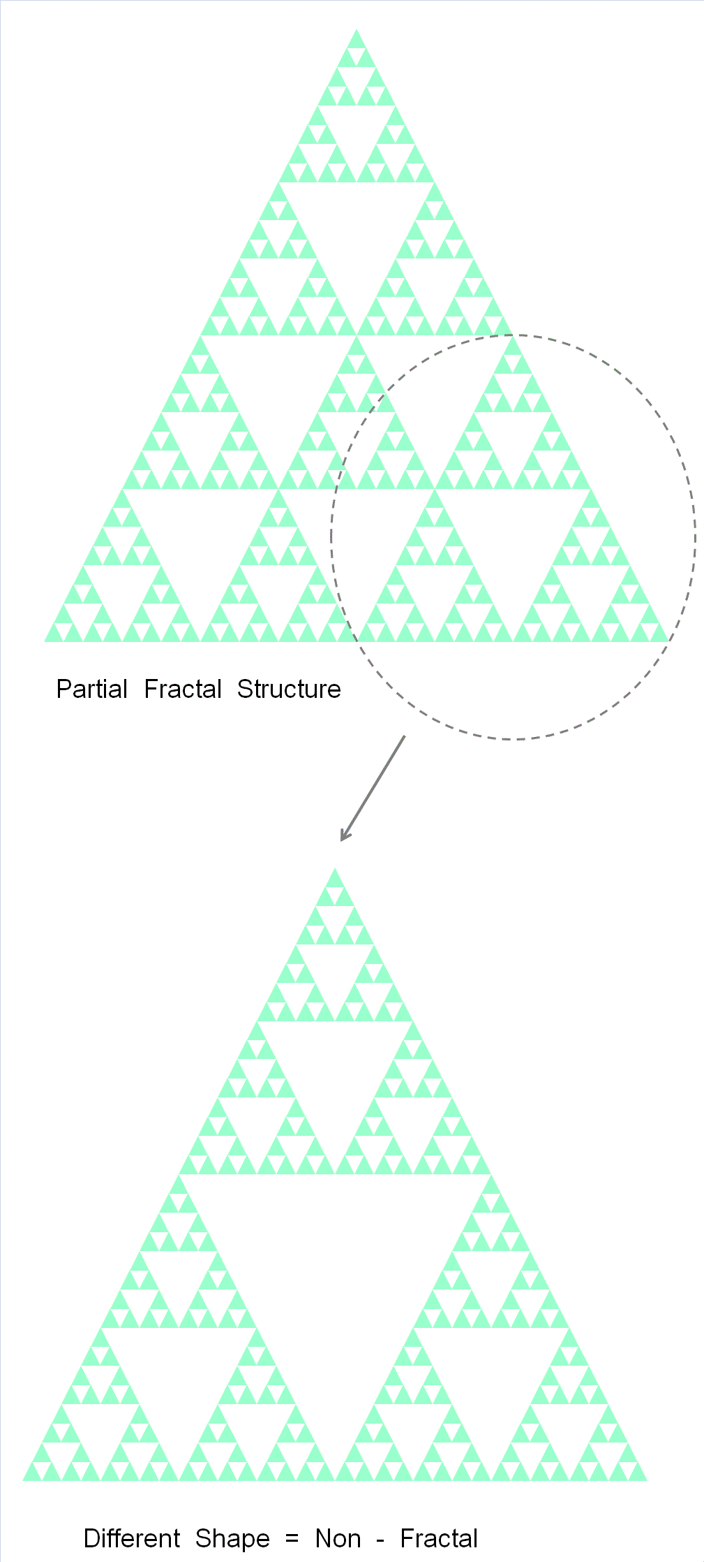
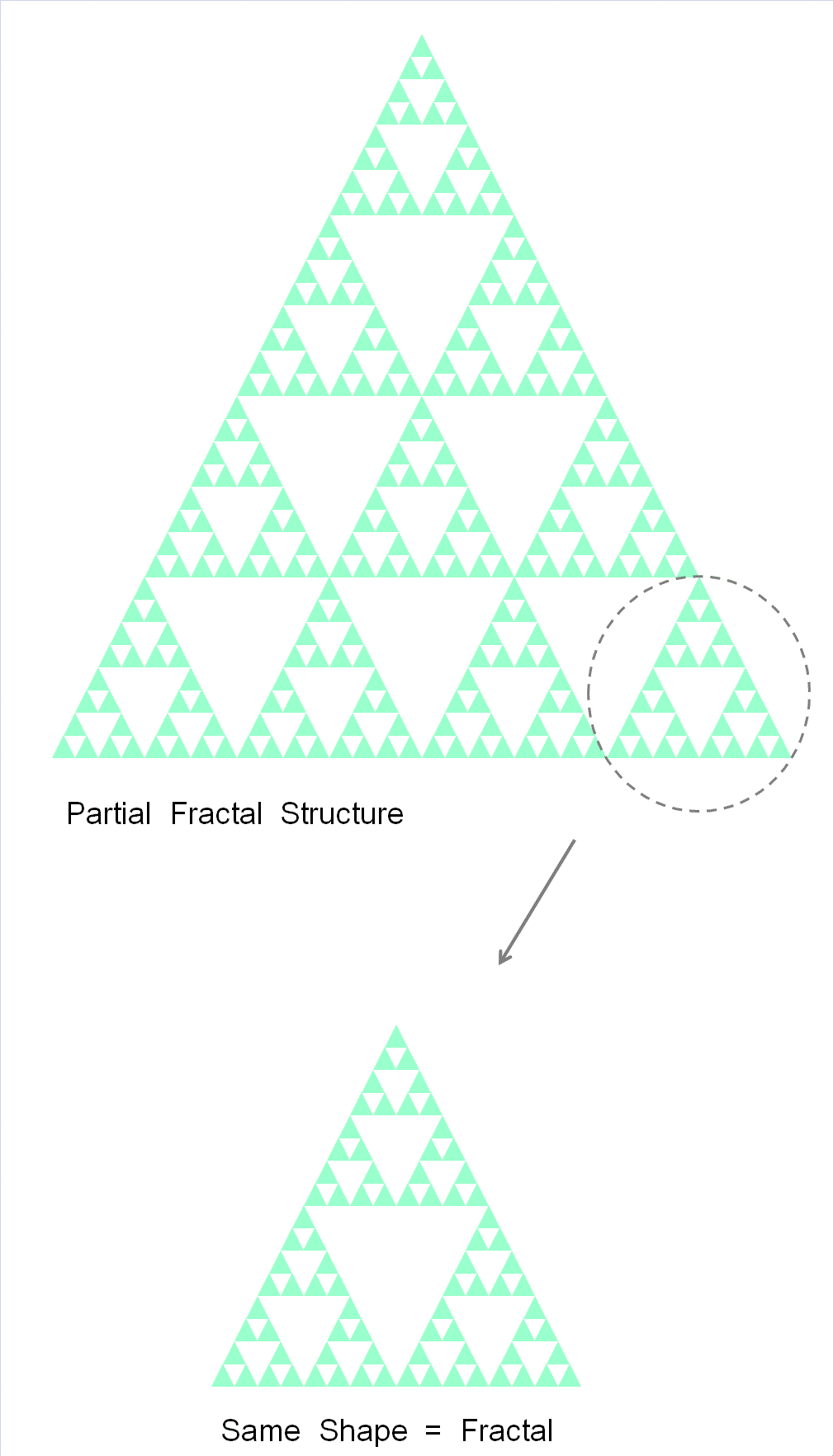
While various definitions of "fractal" exist, for this context, it is defined as a structure that maintains the same pattern regardless of whether the scale is expanded or contracted by an integer factor?for instance, a structure where one small triangle is composed of three even smaller triangles.
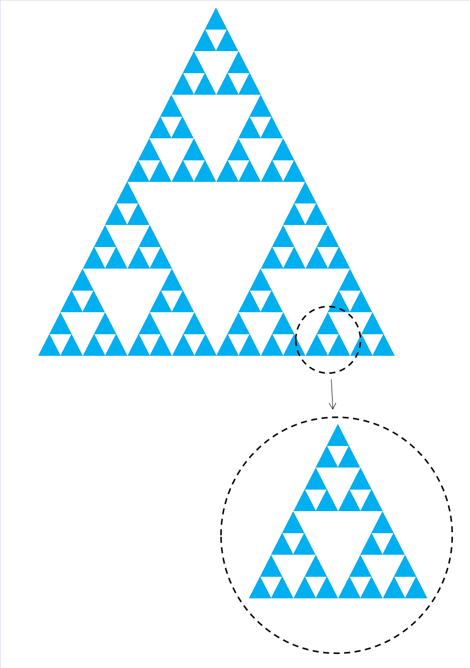
2.6.12.2.1.5.3 Explaining Fractal Structures
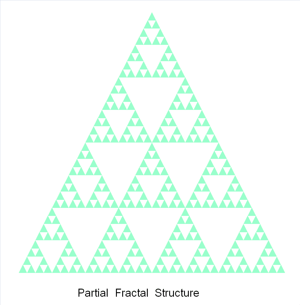
The following provides a general explanation of fractal structures, independent of CDT.
The image below illustrates a typical fractal structure. As long as the magnification is an integer, the same pattern appears regardless of the scale. (In this example, the length roughly doubles at each step. It is assumed that each small green triangle is composed of even smaller triangles.)
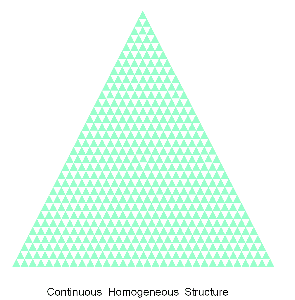
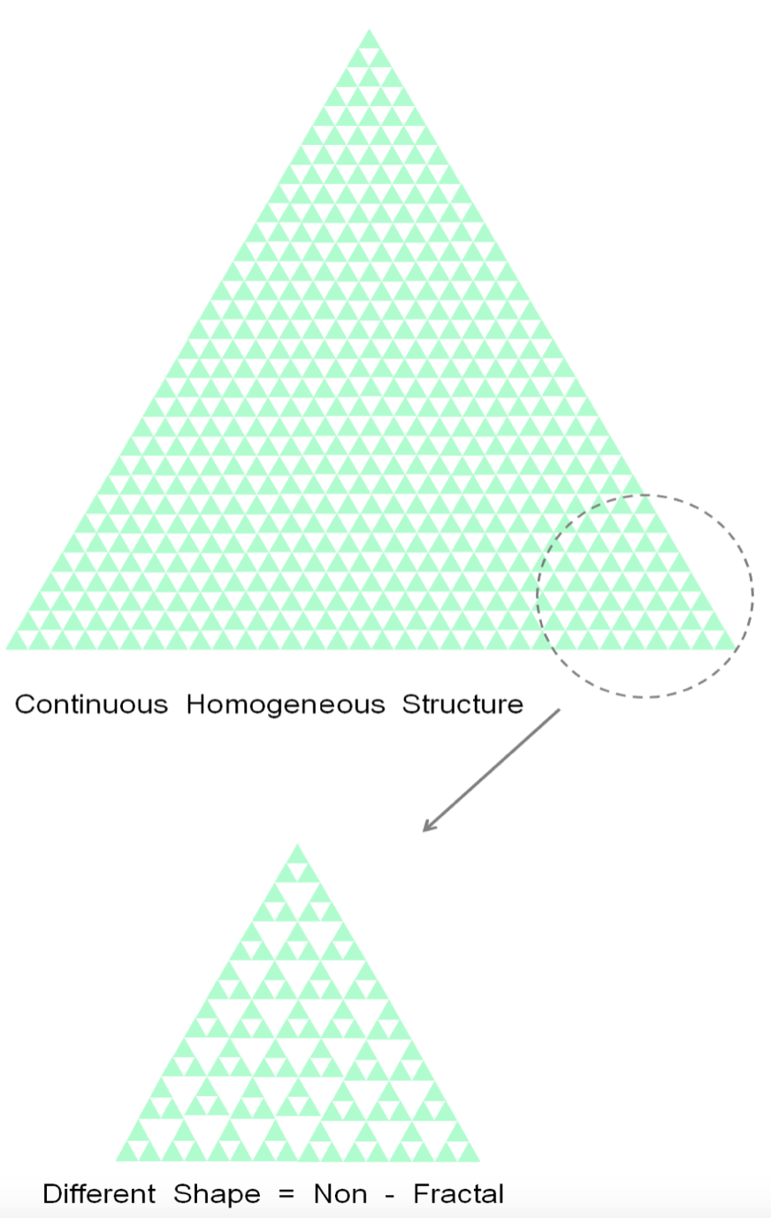
In contrast, the following image represents a "Continuously Homogeneous" state.
Even if one assumes the small green triangles are composed of smaller units, the
pattern does not repeat identically through integer-based scaling. Therefore, this is
not a fractal.
(Note: While Superstring Theory is based on a "continuously homogeneous spacetime" that
assumes no minimum unit, the homogeneous state described here assumes the existence
of a fundamental minimum unit.)
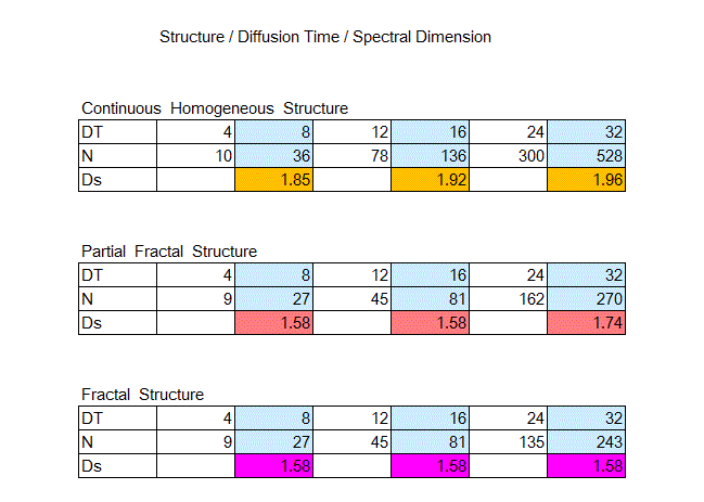
When calculating the spectral dimension, the relationship between
Diffusion Time ($DT$), the number of green triangles ($N$), and the Spectral Dimension ($D_s$) can be summarized as follows. Looking at the values of $D_s$, the continuously homogeneous structure yields a higher dimension, whereas the fractal structure yields a lower dimension.
2.6.12.2.1.5.3 Partial Fractal Structures
However,
the central issue is the phenomenon where dimensionality is high macroscopically but low microscopically. To resolve this, one must consider a "Partial Fractal Structure."
The spectral dimensions of a scale-dependent "Partial Fractal Structure" are summarized below. From a macroscopic perspective, this structure appears continuously homogeneous. However, from a microscopic perspective, it is fractal. Dimensional reduction in CDT suggests that such a partial fractal structure may exist at the Planck scale.
Furthermore, the specific rules or regularities that trigger this reduction at a
certain scale must be investigated. While it is likely linked to the fundamental
minimum unit of the universe, it is also worth considering the possibility of a
pattern where dimensions increase and decrease cyclically.
This concept might be represented by a Layered Fractal Structure.
The next is an example of "Partial Fractal Structure."
A simplified dimensional calculation yields the values shown in the table below. Furthermore, the accompanying diagram provides a conceptual illustration of the Layered Fractal Structure.
2.6.12.2.2 The Holographic Principle, MERA, and Entropic Gravity in 2010 CE
2.6.12.2.2.1 Overview
With the introduction of MERA in 2007 CE and Entropic Gravity in 2010 CE, the Holographic Principle reached its contemporary form. This principle posits that the universe possesses a mechanism akin to a 3D cinematic projector. What humans perceive as a physical, three-dimensional universe is, in essence, a projected image—much like a 3D film.
2.6.12.2.2.2 MERA and the Network of Entanglement
In 2007 CE, Guifré Vidal proposed the MERA (Multi-scale Entanglement Renormalization Ansatz) network as a method for efficiently computing the states of quantum many-body systems (systems involving vast numbers of entangled particles). This network diagram subsequently drew significant attention due to its structural parallels with the Holographic Principle.
A MERA network exhibits a hierarchical structure:
The Base: A dense row of short vertical lines representing individual microscopic quanta (such as spins).
The Upper Layers: Triangles or branching structures merge as they move upward, representing the integration of information through quantum entanglement.
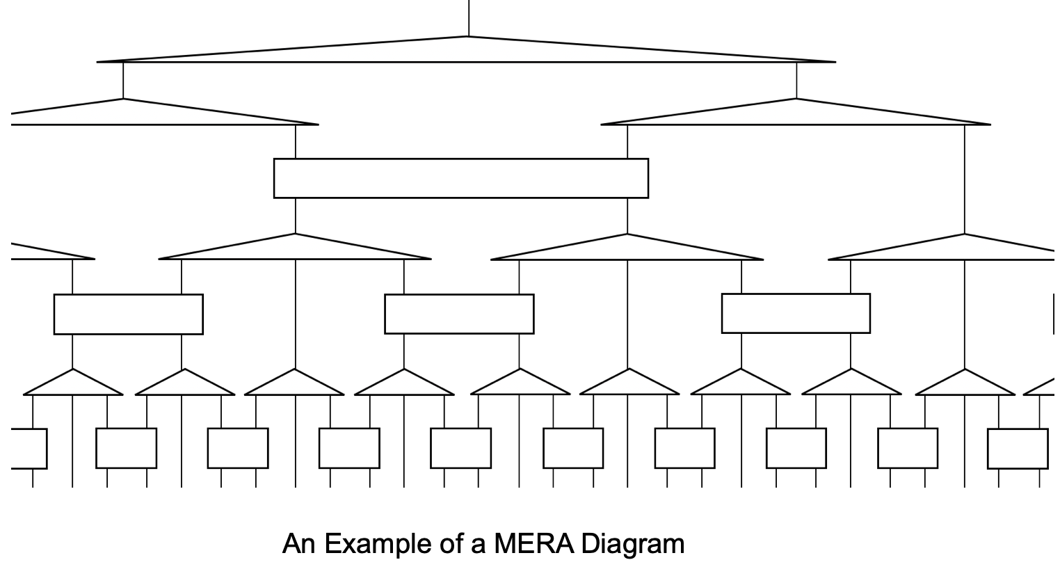
This diagram is considered fundamentally identical to the Poincaré disk in hyperbolic geometry. The base (bottom layer) of the diagram corresponds to the outer boundary of the Poincaré disk, while the upper layers correspond to the region near its center. As the vast amount of digital information located at the base (boundary) moves toward the upper layers (center), it undergoes transformation and integration, eventually evolving into meaningful, synthesized information. Both frameworks are interpreted as mathematical structures that elucidate the operational mechanisms
of the Holographic Principle
*
Poincare Disk Model in Wikipedia"
https://en.wikipedia.org/wiki/Poincar%C3%A9_disk_model
2.6.12.2.2.3 The Core of the Holographic Principle
Proposed around 1993 CE as an extension of the standpoint in (a) Background-Dependent Continuum Holography School,
the Holographic Principle is a concept in quantum gravity stating that "all information contained within a volume of space can be encoded on its lower-dimensional boundary."
This theory suggests that vast amounts of data exist at the far reaches (the surface) of the universe. From this data, visual information is generated and projected inward, creating the 3D reality humans perceive. (The theory remains silent on the origin or "creator" of this 3D projection apparatus.)
*
"Holographic Principle in Wikipedia"
https://en.wikipedia.org/wiki/Holographic_principle
2.6.12.2.2.4 AdS/CFT Correspondence: The Mathematical Sandbox
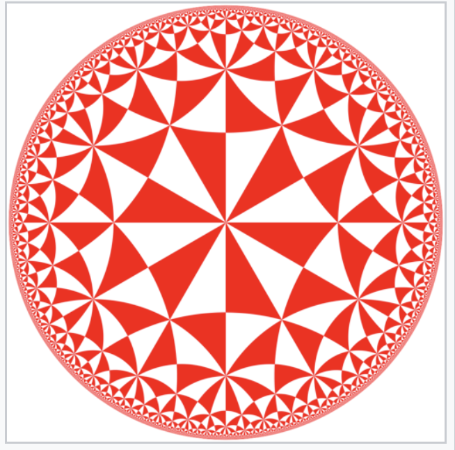
In 1997 CE, Juan Maldacena advanced this principle through the AdS/CFT correspondence. Maldacena utilized a hypothetical "sandbox" model known as Anti-de Sitter (AdS) space, a closed environment shaped like the interior of a massive ball. In this space, light emitted toward the edge cannot escape; it reflects off the boundary as if hitting a "mirrored wall."
Simply put, Anti-de Sitter (AdS) space is a space with negative curvature that expands as one moves away from the center; in two dimensions, it can be likened to the shape of a horse saddle. The Poincaré disk is considered an ideal tool for illustrating this geometric state.
By trapping a black hole inside this "box," Maldacena succeeded in stabilizing and calculating its complex behaviors.
This model demonstrated a one-to-one mathematical correspondence between:
The Interior (3D): Gravitational phenomena.
The Boundary (2D): A gravity-free quantum theory called Conformal Field Theory (CFT).
CFT is characterized by its fractal-like properties, where physical laws remain invariant regardless of whether the scale is zoomed in or out.
In regions like black holes, internal gravity becomes so intense that standard calculations fail. However, this theory allows for calculations on the "boundary wall" where gravity is excluded. The boundary consists of "highly entangled waves of quantum information (fields)."
This gravity-free boundary information is somehow projected into the interior as a three-dimensional world with gravity. For the boundary information to consistently describe the interior across all scales, the boundary must maintain its CFT (fractal) nature.
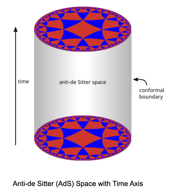
The diagram below illustrates Anti-de Sitter (AdS) space integrated with a time axis. Each cross-sectional disk, representing a specific point in time, is a form of the Poincaré disk.
The theoretical framework posits that the data on the outer boundary includes complex information regarding quantum entanglement. As this information is integrated and projected into the interior, it manifests as gravity. Within this model, each disk represents Anti-de Sitter (AdS) space at a given moment, constructed such that the laws of gravity emerge from the boundary information independently of time.
*
"Anti-de Sitter Space in Wikipedia"
https://en.wikipedia.org/wiki/Anti-de_Sitter_space
2.6.12.2.2.5 The Universe as a Constructed Illusion
Beginning around 2001 CE, theorists such as Andrew Strominger and Leonard Susskind popularized the interpretation that space itself is merely a projection of transformed information from a lower-dimensional surface. This view implies that nothing exists "outside" the boundary.
This leads to the idea that our universe has a spherical boundary at an immense distance, where massive amounts of data are stored, converted, and integrated via quantum entanglement to be projected inward. Even the sensation of gravity is considered a byproduct of this projection. In this framework, the entirety of space is a constructed illusion.
2.6.12.2.2.6 The 3D Movie Analogy
The technology of 3D films, such as Avatar, serves as an effective analogy. The source of the film is digital data—zeros and ones—stored in memory. A computer program processes this data into audio and two distinct 2D visual streams.
Audio: Converted into air vibrations by speakers.
Visuals: Projected as two separate images (for the right and left eyes).
Because the eyes perceive slightly different images, the brain interprets them as a three-dimensional scene. The viewer feels as though a 3D object exists in front of them, but there is no such object—it is a sophisticated illusion. The Holographic Principle suggests our physical reality operates on the same fundamental logic.
*
"Avatar (2009 Film) in Wikipedia"
https://en.wikipedia.org/wiki/Avatar_(2009_film)
Return to the Home Page